


ABSTRACT
We present a survey of the Orion A and B molecular clouds undertaken with the IRAC and MIPS instruments on board Spitzer. In total, five distinct fields were mapped, covering 9 deg2 in five mid-IR bands spanning 3–24 μm. The survey includes the Orion Nebula Cluster, the Lynds 1641, 1630, and 1622 dark clouds, and the NGC 2023, 2024, 2068, and 2071 nebulae. These data are merged with the Two Micron All Sky Survey point source catalog to generate a catalog of eight-band photometry. We identify 3479 dusty young stellar objects (YSOs) in the Orion molecular clouds by searching for point sources with mid-IR colors indicative of reprocessed light from dusty disks or infalling envelopes. The YSOs are subsequently classified on the basis of their mid-IR colors and their spatial distributions are presented. We classify 2991 of the YSOs as pre-main-sequence stars with disks and 488 as likely protostars. Most of the sources were observed with IRAC in two to three epochs over six months; we search for variability between the epochs by looking for correlated variability in the 3.6 and 4.5 μm bands. We find that 50% of the dusty YSOs show variability. The variations are typically small (∼0.2 mag) with the protostars showing a higher incidence of variability and larger variations. The observed correlations between the 3.6, 4.5, 5.8, and 8 μm variability suggests that we are observing variations in the heating of the inner disk due to changes in the accretion luminosity or rotating accretion hot spots.
Export citation and abstract BibTeX RIS
1. INTRODUCTION
Strewn across the constellation Orion are the most massive and active molecular clouds within 500 pc of the Sun. These clouds host the nearest sites of high-mass star formation as well as thousands of young low-mass stars. They are important laboratories for studying star and planet formation in a range of environments, from near isolation, to small groups, and finally to massive clusters. The large angular (and spatial) size of the Orion molecular clouds, which extend 12° (90 pc) on the sky, necessitates the use of wide-field surveys to observe the clouds in their entirety. We present here the first wide-field, 2''–5'' resolution, mid-IR survey of the clouds using the InfraRed Array Camera (IRAC) and the Multiband Imaging Photometer for Spitzer (MIPS) on board the Spitzer Space Telescope. With these data, we have undertaken a spatially unbiased survey for dusty young stellar objects (YSOs) associated with the Orion clouds.
The cloud complex is composed of two distinct molecular clouds, the Orion A and Orion B clouds, with a total mass in excess of 2 × 10⁵ M☉ (Wilson et al. 2005). The Orion A cloud contains the Orion Nebula and the first known embedded cluster, the Orion Nebula Cluster (hereafter ONC; Trumpler 1931; Baade & Minkowski 1937; Zinnecker et al. 1993; O'Dell et al. 2008). The ONC is one of the two richest young stellar clusters currently known within 1 kpc of the Sun (Porras et al. 2003; Lada & Lada 2003; Allen et al. 2012). This cluster has emerged as an important laboratory for understanding the initial mass function (Hillenbrand 1997; Luhman et al. 2000; Muench et al. 2002), the evolution of disks around young stars (Hillenbrand et al. 1998; Lada et al. 2000, 2004), and the structure and kinematics of young clusters (Hillenbrand & Hartmann 1998; Fűrész et al. 2008; Tobin et al. 2009). The OMC-2/3 star-forming region (which may be considered part of the ONC cluster; Peterson & Megeath 2008) and the L1641 molecular cloud (Allen & Davis 2008) are also part of the Orion A cloud. The Orion B cloud contains the NGC 2024 H ii region as well as the NGC 2023, 2068, and 2071 reflection nebulae. All of these regions also contain clusters or groups of young stars (Lada et al. 1991; Chen & Tokunaga 1994; Allen & Davis 2008; Peterson & Megeath 2008; Meyer et al. 2008; Flaherty & Muzerolle 2008). Directly to the north of the Orion B cloud is the Lynds 1622 cloud. Since this cloud appears to be at the same distance as the Orion B cloud, we include Lynds 1622 as part of Orion B (Reipurth et al. 2008; Bally et al. 2009). Very long baseline interferometry parallax measurements of stars and masers in the Orion Nebula give an average distance of 420 pc (Sandstrom et al. 2007; Menten et al. 2007; Hirota et al. 2007). Although there is evidence that the distances to the various clouds in Orion may vary by as much as 100 pc (Wilson et al. 2005), we adopt 420 pc as the distance to the entire cloud complex in our analysis.
Stellar photometry with the IRAC and MIPS instruments can be used to detect excess infrared emission due to starlight reprocessed by dust grains in disks and envelopes (Megeath et al. 2004; Allen et al. 2004, 2007; Muzerolle et al. 2004; Whitney et al. 2004; Hartmann et al. 2005). Many of the dusty YSOs identified by their mid-IR (⩾3.6 μm) emission do not exhibit substantial excess emission in the near-IR (1–2.2 μm) bands, which are often dominated by the photospheric emission from the star (Gutermuth et al. 2004). In contrast, at mid-IR wavelengths the emission from disks and envelopes exceeds that from the star (Whitney et al. 2003; D'Alessio et al. 2006). In this paper, we identify young stars with disks and protostars using a suite of color–color diagrams and color–magnitude diagrams constructed from the merged 3–24 μm photometry of the IRAC and MIPS instruments of Spitzer and the near-IR photometry from the Two Micron All Sky Survey (2MASS) point source catalog (Gutermuth et al. 2009; Kryukova et al. 2012). With this merged photometry, we map the spatial distribution of dusty YSOs in a 14 deg2 survey field covering the Orion A and B molecular clouds.
By identifying such objects through their infrared excesses, we can study for the first time the extended spatial distribution of protostars and young pre-main-sequence stars with disks in the entire cloud complex. In contrast to previous papers that mapped the distribution of YSOs using the surface density of near-IR sources (Lada et al. 1991; Carpenter 2000), we can identify individual YSOs irrespective of whether they are found in clusters or in isolation. The resulting census of dusty YSOs provides a more representative portrait of the full range of star-forming environments present in the Orion clouds. It also provides the means to detect variability in the emission from dusty disks and envelopes between the two to three epochs of IRAC photometry. When compared to an independent estimate of the number of pre-main-sequence stars without disks, the census can be used to estimate the fraction of pre-main-sequence stars that have circumstellar disks and the fraction of young stars in their protostellar phase.
This contribution is the first of two papers presenting the results of the Spitzer Orion Survey. In this paper, we describe the construction of the catalog of all point sources in the surveyed fields and the identification of dusty YSOs in the catalog. We then show the distribution of both pre-main-sequence stars with disks and protostars in the Orion clouds. Since much of the IRAC data were taken in two to three epochs over an eight month period, we also use these data to examine the variability of the YSOs. This work complements the warm mission YSOVAR variability survey of the ONC by searching for variability in a larger sample of YSOs and by measuring the variability in all four IRAC wavelength bands (Morales-Calderón et al. 2011). In addition, we present a new means for characterizing the spatially varying completeness of point sources in nebulous fields.
In a second paper, we will correct for the spatially varying incompleteness found in the YSO catalog and map the density of dusty YSOs across the clouds. Using the corrected distribution of YSOs, we will examine the demographics of protostars and young stars with disks in the diverse environments found within the Orion molecular clouds, compare the Orion clouds to other nearby molecular clouds, study the structure of embedded clusters, and estimate the fraction of young stars with disks within the clouds.
In addition, this paper has two companion papers that use the YSO catalog extracted from the Spitzer Orion Survey: a study of the relationship between stellar and gas surface densities in molecular clouds (Gutermuth et al. 2011) and a comparative study of protostellar luminosity functions in nine nearby molecular clouds (Kryukova et al. 2012). Together, these papers comprise an analysis of many facets of the Spitzer Orion Survey, including the mechanisms for YSO variability, the demographics of star formation, the properties of embedded clusters, and the influence of environment on star and planet formation.
2. THE SPITZER ORION POINT SOURCE CATALOG
The Orion clouds were surveyed with the IRAC and MIPS instruments on board the Spitzer Space Telescope (Fazio et al. 2004; Rieke et al. 2004). This paper describes the extraction of point source photometry from the survey in the four IRAC bands and the MIPS 24 μm band and the initial results derived from that photometry. In this section, we discuss the observations, the data reduction, the identification of point sources, and the determination of photometric magnitudes in the Spitzer 3.6, 4.5, 5.8, 8, and 24 μm bands. We then overview the basic properties of the resulting point source catalog.
2.1. IRAC Observations
The IRAC observations were taken as part of the Guaranteed Time Observation (GTO) programs PID 43, 50, 30641, and 50070. Table 1 contains a complete summary of the IRAC observations. The maps were made using a triangular grid of pointing centers in celestial coordinates. Since this grid was fixed to the celestial sphere, the map could be adjusted to follow the contours of the molecular cloud. The triangular grid was designed so that the observations could be executed at the full range of possible spacecraft orientations without holes in the coverage. Each field was observed in two epochs scheduled during consecutive visibility periods; this ensured that the detector arrays were rotated by as much as 180° between the epochs. The rotation between the two epochs effectively swapped the positions of the two spatially offset IRAC field of views (FOVs; i.e., the 3.6/5.8 μm and the 4.5/8 μm FOVs), thus providing full four-band coverage over most of the survey area. The rotation also facilitated the removal of bright source artifacts in the data.
Table 1. IRAC Observations
| Field Name | Frame | No.a of | Total Int. | Fieldb | 1st Epoch | 2nd Epoch | PID |
|---|---|---|---|---|---|---|---|
| Time (s) | Dithers | Time (s) | (deg2) | ||||
| ONC | 12 HDR | 4 | 41.6 | 1.33 | 2004 Mar 9 | 2004 Oct 12 | 43 |
| L1641 | 12 HDR | 4 | 41.6 | 2.71 | 2004 Feb 16–18 | 2004 Oct 8, 27c | 43 |
| Ori A ext. | 12 HDR | 4 | 41.6 | 1.91 | 2007 Oct 21 | 2008 Apr 9–10 | 30641 |
| κ Ori ext.d | 12 HDR | 4 | 41.6 | 1.21 | 2009 Mar 21–22 | ... | 50070 |
| ONC centerd | 2 | 24 | 28.8 | 0.08 | 2004 Oct 27 | ... | 50 |
| NGC 2024/23 | 12 HDR | 4 | 41.6 | 1.20 | 2004 Feb 17 | 2004 Oct 27 | 43 |
| NGC 2024d | 2 | 24 | 28.8 | 0.04 | 2004 Oct 8 | ... | 50 |
| NGC 2024 ext. | 12 HDR | 4 | 41.6 | 0.07 | 2007 Mar 30 | 2007 Oct 16 | 30641 |
| NGC 2068/71 | 12 HDR | 4 | 41.6 | 1.10 | 2004 Mar 7 | 2004 Oct 28 | 43 |
| L1622 | 12 HDR | 4 | 41.6 | 0.23 | 2005 Oct 27 | 2006 Mar 25 | 43 |
| Ori B fil. | 12 HDR | 4 | 41.6 | 0.36 | 2007 Mar 29–30 | 2007 Oct 16–17 | 30641 |
| Reference 1d | 12 HDR | 4 | 41.6 | 0.13 | 2005 Oct 26–29 | 43 | |
| Reference 2a | 12 HDR | 4 | 41.6 | 0.16 | 2007 Oct 16 | 30641 | |
| Orion A total | 12 HDR | 4 | 41.6 | 5.86 | ... | ... | ... |
| Orion B total | 12 HDR | 4 | 41.6 | 2.96 | ... | ... | ... |
Notes. aNumber of pointings per map positions for both epochs combined. bArea with complete four-band coverage except for the 2 s exposures, where we state the single-band coverage fields. cThe two dithers of the second epoch observation were observed on separate dates. dOnly one epoch was observed.
Download table as: ASCIITypeset image
The 12 s high dynamic range (HDR) mode was used; this produced two frames with integration times of 0.4 s and 10.4 s (corresponding to frame times of 0.6 and 12 s). At every map position, two dithered observations were obtained during each epoch. Thus, for most positions, the total integration time is at least 41.6 s per band for the long HDR frames and 1.6 s for the short HDR frames. However, due to the rotation of the two FOVs between the two epochs, many positions at the edges of the map have an integration time of 20.8 s per band for the long HDR frames and 0.8 s for the short HDR frames.
In Figure 1, the surveyed FOVs are shown overlaid on an extinction map of the Orion clouds from Gutermuth et al. (2011). The Orion cloud complex consists of two distinct giant molecular clouds, Orion A and Orion B, as shown in 12CO and 13CO surveys of this region (Bally et al. 1987; Miesch & Bally 1994; Wilson et al. 2005). The Orion A cloud was surveyed in one contiguous 4.04 deg2 map extending from NGC 1977 down through the L1641 dark cloud. The survey field was constructed to follow the distribution of 13CO emission in the Bell Labs survey of Orion A (Bally et al. 1987). The survey was later extended to fully map the ONC. Subsequent extinction maps of the Orion clouds showed the Orion A cloud extending to a declination of −10° (κ Ori extension in Figure 1; Carpenter 2000); the survey was expanded again to include this southern extension of the cloud. In addition to the L1641 dark cloud, the 5.9 deg2 map of Orion A also contains the L1640 dark cloud (part of the ONC region) and the L1647 dark cloud (which we include as part of the L1641 region). The Orion B map was broken into three fields centered on the regions of strong 13CO emission (Miesch & Bally 1994): a 1.27 deg2 field covering the NGC 2024 and NGC 2023 nebulae in L1630, a 1.1 deg2 field covering the NGC 2068 and NGC 2071 nebulae in L1630, and a 0.36 deg2 field covering a region of bright 13CO emission in between the NGC 2068/2071 and NGC 2024/2023 fields (hereafter Orion B filament). In addition, a 0.23 deg2 field covering the dark cloud L1622 was observed; in this paper, we consider L1622 to be part of the Orion B cloud (Bally et al. 2009).

Figure 1. Coverage of the Spitzer Orion cloud survey. The grayscale image is an extinction map of the Orion region made from the 2MASS PSC (Gutermuth et al. 2011). Left: the fields surveyed with IRAC. The fields are labeled by the designations used in the text, these labels are drawn from their constituent star-forming regions, their designation in the Lynds dark nebulae catalog, or their apparent proximity to a prominent star (κ Ori). In the case of Orion A, these fields merge into one contiguous field. The extensions of the NGC 2024, ONC, and L1641 fields are also identified. To extend the completeness of our YSO sample in the Orion B cloud, we also mapped a small, clumpy filament separate from the major star-forming regions (denoted "filament"). Flanking the Orion A cloud are five fields placed to measure the density of young stellar objects and contaminating objects outside the cloud, but within the Orion OB1 association. To the east are three additional reference fields; these are designed to measure density of contaminating objects outside the Orion OB1 association. The red/cyan boxes outline the mosaics obtained in the two IRAC fields of view using the 2 s frame time. Right: the fields surveyed with MIPS. The five major fields are indicated; the Orion B filament and NGC 2068/2071 fields overlap. The initial fields are outlined in green, the extension fields are outlined in red. The saturated regions of the MIPS data in the Orion Nebula and NGC 2024 are outlined in green.
Download figure:
Standard image High-resolution imageIn program PID 50, the NGC 2024 nebula and Orion Nebula were observed with 1.2 s integration time frames (corresponding to a frame time of 2 s) to obtain high-signal-to-noise ratios in regions toward which the 10.4 s frames were saturated by bright nebulosity. Toward the Orion Nebula, the map consisted of a 3 × 4 rectangular grid in spacecraft coordinates with 270'' offsets between pointing centers. Toward NGC 2024, a 2 × 3 rectangular grid in spacecraft coordinates was made with the same offsets. In both maps, 24 dithered 2 s frames were obtained per map position for total integration times of 28.8 s per band.
A total of eight reference fields were also observed; these covered a total of 0.41 deg2 in all four bands (Figure 1). For each field, a single epoch observation with four dither positions was executed; the typical integration time was 41.6 s per band. Five of the fields were observed in 2005 October (PID 43); these consist of four fields on either side of the ONC and one field targeting a small cloud east of Orion A detected by Bally et al. (1987). The remaining fields, all of which are found to the east of the cloud complex, were observed in 2007 October (PID 30641).
2.2. MIPS Observations
The MIPS observations were obtained from GTO programs PID 43, 47, 58, 30641, and 50070. The observations are tabulated in Table 2 and displayed in Figure 1. The Orion A cloud was mapped in six distinct fast scan maps: one covering the ONC (Table 2), one extending the ONC map to the north, and three covering L1641 and one covering the part of the cloud adjacent in the sky to the star κ Ori. The cross-scan steps were 148'' or 160'', resulting in a typical integration time of 30 s per pixel. The combined map covered 11.43 deg2. The Orion B cloud was mapped using four individual scan maps. The NGC 2068/2071 region was mapped using medium-rate scans and 160'' cross-scan offsets, giving a typical integration time of 80 s per pixel. The NGC 2024/2023 region and Orion B filament were mapped with fast scans and either 148'' or 160'' cross-scan steps; the resulting integration time was 30 s. The result was two contiguous maps: a 2.58 deg2 map including NGC 2068/2071 and the filament, and a 2.04 deg2 map of NGC 2024/2023. Finally, a field covering 0.31 deg2 toward L1622 cloud was mapped using medium-rate scans and 302'' cross-scan offsets with a typical integration time of 40 s.
Table 2. MIPS 24 μm Observations
| Field Name | Scan Rate | Cross Scan | No. of | Total Int. | Field | Epoch | PID |
|---|---|---|---|---|---|---|---|
| Offset ('') | Frames | Time (s) | (deg2) | ||||
| ONC | fast | 160'' | 6 | 30 | 2.18 | 2004 Mar 20 | 58 |
| ONC Ext. | fast | 160'' | 6 | 30 | 2.28 | 2008 Apr 19 | 30641 |
| L1641a | fast | 148'' | 6 | 30 | 5.35 | 2005 Apr 2 | 47 |
| κ Orib | fast/medium | 148''/302'' | 6/20 | 30/40 | 3.77 | 2008 Nov 26–27 | 50070 |
| NGC 2024/23 | fast | 148'' | 6 | 30 | 2.04 | 2005 Apr 3 | 47 |
| NGC 2068/27 | medium | 160'' | 20 | 80 | 0.97 | 2004 Mar 15 | 58 |
| L1622 | medium | 302'' | 20 | 40 | 0.31 | 2005 Nov 4 | 43 |
| Ori B fil. | fast | 160'' | 6 | 30 | 1.94 | 2008 Apr 16 | 30641 |
| Orion A total | 11.43 | ||||||
| Orion B total | 4.93 |
Notes. aThis field was mapped in three separate scan maps. bThis field was combined from fast- and medium-rate scan maps.
Download table as: ASCIITypeset image
2.3. IRAC Data Reduction
The data were mosaicked using the custom IDL package Cluster Grinder (Gutermuth et al. 2009). The input images were basic calibrated data (BCD) data processed with the Spitzer Science Pipeline. The BCD data pipeline versions included s14, s17, and s18. Cluster Grinder first prepares the BCD images for mosaicking by matching the background of adjacent images, executing cosmic-ray masking using overlapping images, and ameliorating artifacts due to column pull-down, banding, muxbleed and residual bandwidth effects (see the chapter on IRAC in the Spitzer Observation Manual for a discussion of these artifacts).
The cosmic-ray rejection is done by comparing overlapping pixels in the four or more frames covering a given mosaic pixel. Pixels which differ by more than 10 median absolute deviations from the median value are masked out of the mosaic. On the outskirts of the mosaics there are sometimes only two overlapping pixels due to the FOV rotation between epochs; in these cases we increase the redundancy by including multiple pixels from each overlapping image. Specifically, we include pixels that are in the same row or column and are directly adjacent to each overlapping pixel resulting in 10 pixels used in the cosmic-ray rejection for each mosaic pixel. Pixels that deviate by more than 20 median absolute deviations from the median value of the 10 pixels are then masked. For the 1.2 s imaging of the ONC and NGC 2024, the high level of redundancy will translate into improved cosmic-ray rejection compared to the longer integration time mosaics.
The data units were converted from the native BCD units of MJy sr−1 into DN by dividing by the conversion factor given in the BCD header ("FLUXCONV") and then multiplying by the integration time. Cluster Grinder then uses the refined WCS information in the BCD image headers to register the images to the mosaic grids and interpolate the BCD images onto the mosaic grid, which had an identical pixel scale to the BCD data. The mosaic pixels were given the value of the average interpolated BCD images weighted by a bad pixel mask.
For the data taken in HDR mode, two mosaics were produced for each wavelength band: one from the 10.4 s integration time data and the other from the 0.4 s integration time data. These are then combined into a single mosaic by replacing all saturated pixels in the 10.4 s mosaic with the pixel values from the 0.4 s mosaic scaled to a 10.4 s integration time. For the 1.2 s data, a single mosaic was produced for each wavelength band.
2.4. The Generation of the 2MASS and IRAC Point Source Catalog
The point sources on the HDR combined mosaics were identified using PhotVis v1.10 (Gutermuth et al. 2008). PhotVis convolved the mosaics with a sunken Gaussian with an FWHM similar to that of a point source (2 pixels). It then identified all sources in the convolved image where the peak was seven times the rms of the pixel values in a 10 × 10 region centered on the peak. Since regions with bright structured nebulosity have higher rms values, this approach dramatically reduced the number of nebular knots misidentified as stars. The point sources identified on each mosaic were then inspected by eye using PhotVis and all obvious artifacts misidentified as point sources remaining in the data were removed at this stage. In addition, a small number of sources that were missed by PhotVis due to confusion with nebulosity were added. Photometric magnitudes were extracted with PhotVis using a 2 pixel radius aperture and an annulus from 2 to 6 pixels to estimate the sky contribution. The zero points were 19.6642, 18.9276, 16.8468, 17.3909 (for units of DN s−1) and aperture corrections were 1.213, 1.234, 1.379, and 1.584 for the 3.6, 4.5, 5.8, and 8 μm bands, respectively (Reach et al. 2005). The uncertainties for each of the four IRAC bands were calculated by the IDL Astronomy Library routine aper.pro by combining the estimated shot noise from the source, the uncertainty in the background estimation, and the measured standard deviation in the sky annulus (PhotVis incorporates routines from the IDL Astronomy Library of Landsman 1993).
At this point, an initial point source catalog was generated using the bandmerging routine within Cluster Grinder. The routine employs the following procedure. First, each 3.6 μm point source was associated with the nearest point source in the longer wavelength bands as long as they were separated by ⩽1''. If the nearest point source was beyond 1'', no association was made and the source would have a detection only in the 3.6 μm band. This procedure was repeated in turn for the 4.5, 5.8, and 8 μm point sources that were not previously merged with a shorter wavelength band. The point sources were then associated with the nearest 2MASS point source as long as the 2MASS source was within a separation of 1 2. The final R.A. and declination pair chosen was that given by the first wavelength band with an uncertainty ⩽0.25 mag in the following progression: 4.5 μm, 3.6 μm, 8 μm, 5.8 μm, and 2MASS. The end product was a catalog of point sources with R.A., declination, photometric magnitudes for all seven bands, and the uncertainties in all seven bands.
Photometric magnitudes of stars observed at multiple positions on flat-fielded BCD images show variations of 5% (see IRAC chapter of Spitzer Observing Manual). To correct for these variations and to search for photometric variability, final photometric magnitudes were then derived from the individual BCD images using the coordinates in the point source catalog derived from the mosaics. These final magnitudes were obtained for all point sources identified in the mosaics with uncertainties ⩽0.25 mag in one of the four IRAC bands. The steps of this process were the following. First, each frame containing a given source was identified, divided by the conversion factor of MJy sr−1 over DN s−1 (i.e., "FLUXCONV"), and then multiplied by the integration time to convert the units into DN. These frames were then corrected for column pull-down, banding, muxbleed, and residual bandwidth effects using custom IDL programs developed for Cluster Grinder. Finally, the R.A. and declination pair of each source, as determined from the mosaics, was converted to pixel coordinates in the BCD images using the refined WCS information in the BCD headers. Aperture photometry was extracted at these positions using aper.pro with an aperture of 2 pixels and a sky annulus of 2–6 pixels. The zero points and aperture corrections were identical to those used for the mosaics. The photometry was then further corrected using the array location dependent photometric corrections given by the Spitzer Science Center;11 these corrections account-for the 5% variation in point source photometry observed across the BCD images. We note that point response function (hereafter PRF) fitting was not used due to the difficulty in taking into account the variations of the IRAC PRF across the focal plane. (The PRF is the point-spread function convolved with the pixels response function.)
The photometry was extracted independently from both the 10.4 s and 0.4 s frames. Thus, each point source was typically measured eight times (four dithers and two integration times), although in many cases the sources were not detected at the shorter integration time. For the ONC and NGC 2024 observations with 1.2 s frames, each point source was measured independently for all 24 dithers. The photometry of each point source was collated as a function of Julian date for all three integration times. Magnitudes were calculated for all sources that were detected in two or more images of the same integration time. For each combination of source, wavelength band, and integration time, the median magnitude was tabulated using the average of the middle two magnitudes when an even number of photometry values were present (if there were only two photometry values, the average of those two values was used). The use of the median value eliminates the impact of cosmic-ray strikes as long as there were three or more dithers and only one dither out of the three was affected. Each of the median magnitudes was assigned an uncertainty equal to (∑Ni = 0σi2/N2)1/2 where σi was the uncertainty of the ith magnitude and N was the total number of magnitudes for a given source, band, and frame time combination. To construct the final table of photometry, the 10.4, 1.2, and 0.4 s data were compared, and the highest signal-to-noise photometry achieved without saturation was adopted. The integration time at which a given point source would saturate was determined from the peak pixel value of that point source in the HDR combined mosaics.
Comparison of the photometry determined directly from the mosaics with that measured from the individual BCD frames showed a systematic offset. The median values of the differences of the magnitudes, mmosaic − mBCD, were 0.02, 0.03, and 0.03 mag for the 3.6, 4.5, and 8 μm bands, but was −0.05 mag for the 5.8 μm band. This resulted in slightly red [5.8] − [8] colors even for pure, Vega-like photospheres. To remove this offset, we corrected the magnitudes in the 5.8 μm band using the average difference between the 5.8 μm band offset and the offsets in the other bands. The correction was applied with the equation m(5.8 μm) = mBCD(5.8 μm) − 0.077 mag.
A final photometric catalog of IRAC and 2MASS photometry was then created by replacing the photometry from the mosaics with the median value of the individual frame photometry. Note that a photometric magnitude in a given band would be replaced only if the uncertainty for the mosaic photometry was ⩽0.25 mag in that band. Otherwise, the magnitude for that band was set to −100 and the uncertainty to 10. Although the 0.25 mag limit might be considered only a 4σ detection, all of the sources were previously found by PhotVis by showing a peak pixel value 7σ above the noise. Furthermore, we apply more stringent limits to the photometry when we search for YSOs.
2.5. The Reduction of the MIPS 24 μm Data and the Generation of the 24 μm Point Source Catalog
The MIPS 24 μm data were reduced, calibrated, and mosaicked using the MIPS instrument team's Data Analysis Tool (Gordon et al. 2005). The resulting MIPS mosaics have a pixel size of 1245 and units of DN s−1 det pix−1 (where det pix is a detector pixel). Point source identification and aperture photometry was first performed with PhotVis. As was done for the IRAC data, PhotVis convolved the mosaics with a sunken Gaussian having a 4.5 mosaic pixel FWHM and then identified all sources in the convolved image where the peak pixel value was seven times the rms of the pixel values in a 10 × 10 region centered on the peak. An aperture of 5 pixels (6225) and a sky annulus extending from 12 (1494) to 15 (18675) pixels were used. We adopted a zero-point magnitude of 16.05; this was calculated using a mosaic pixel that was half the diameter of a detector pixel, a calibration factor of 6.4 × 10⁻⁶ Jy per DN s−1 det pix−1 (again, det pix is a detector pixel), and a zero magnitude flux in the MIPS 24 μm band of 7.17 Jy. In addition, an aperture correction was included in the zero-point magnitude, which consisted of two first parts. First, we multiplied the signal in the aperture by 1.146; this is the correction from a 12 pixel aperture to infinity (Engelbracht et al. 2007). Furthermore, we applied the aperture correction between the 5 pixel aperture used in our photometry and the 12 pixel aperture. This was determined by comparing the photometry in 5 and 12 pixel apertures for a sample of bright, isolated, and unsaturated stars in our sample; the resulting correction was −0.428 mag.
Given that that the MIPS PSF has an FWHM more than twice that of the IRAC PRF, it was necessary to revise the photometry using PSF-fitting photometry to minimize the effect of confusion with other sources and nebulosity. The extraction of the MIPS photometry using PSF-fitting is described in Kryukova et al. (2012). The PSF photometry was calibrated using the aperture photometry obtained for the stars used to construct the reference PSF. Thus, it will have the same calibration as the aperture photometry described above.
There are two regions of spatially extended saturation in the MIPS 24 μm survey where point sources could not be detected. The largest region of saturation is found in the Orion Nebula at the center of the ONC. The saturation encompasses the Trapezium as well as the region surrounding BN/KL. This region has been recently mapped at 6–37 μm with FORCAST on SOFIA by Shuping et al. (2012). The other region of extended saturation is located in the NGC 2024 nebula and contains the exciting star of NGC 2024, IRS 2b (Bik et al. 2003).
Finally, the MIPS point sources were merged with the combined 2MASS and IRAC point source catalog. The R.A. and declination of point sources in the IRAC point source catalog were compared to the positions of the MIPS 24 μm point sources. The MIPS magnitudes and uncertainties were then assigned to the nearest IRAC point sources if they were separated by ⩽25. If there was no IRAC photometry within this limit, the MIPS coordinates, magnitudes, and uncertainties were added to the point source catalog as a new source.
2.6. The Spitzer Point Source Catalog and Its Completeness
The final point source catalog contains 298,405 sources that are detected in at least one of the IRAC bands or in the MIPS 24 μm band. The magnitude uncertainties for the point source photometry are displayed in Figure 2. The uncertainties in all eight bands follow the expected upward sloping curve with the uncertainties increasing with increasing magnitude; however, the uncertainties in the IRAC bands show a large scatter for a given magnitude. The reason for this spread is that the uncertainties depend not only on the magnitude of the source, but also their location. Sources located toward bright, structured nebulosity or in regions crowded with other point sources show higher uncertainties than sources with equal magnitudes in regions without bright nebulosity or crowding.

Figure 2. Uncertainties as a function of magnitude for the final adopted photometry in the three 2MASS bands, the four IRAC bands, and the MIPS 24 μm band. The colors indicate the RMEDSQ for a given source in the 8 μm band (the 8 μm band exhibits the brightest nebulosity of the four IRAC bands): blue indicates RMEDSQ < 30, green indicates 30 ⩽ RMEDSQ < 100, and red indicates RMEDSQ ⩾ 100. In the identification of YSOs, only magnitudes with uncertainties less than 0.1 mag are used for the J, H, Ks, [3.6], and [4.5] bands and with uncertainties less than 0.15 mag in the [5.8] and [8] bands.
Download figure:
Standard image High-resolution imageTo assess the dependence of the measured uncertainties on the presence of nebulosity and nearby point sources, we determine the root median square deviation (hereafter RMEDSQ) of the pixel values in an annulus centered on the point source. The RMEDSQ for a given star is given by

where i0 and j0 are the pixel coordinates of the source, and i, j are the pixels that are found in an annulus centered on the source. For the IRAC photometry, the annulus typically extends from 6 to 11 pixels (72–132). For bright stars, fluctuations in the PRF may dominate the RMEDSQ in this annulus. To ensure that the PRF itself does not contribute to the RMEDSQ, the radius of the annulus is extended to larger radii until variations in the PRF make a negligible contribution to the RMEDSQ. The maximum allowed size of an annulus is from 45 to 50 pixels (54''–60''). Since the units of our mosaics are DN, the resulting RMEDSQ are in units of DN. For the MIPS photometry, the annulus also extends from 6 to 11 pixels (747–13695). Again, the radius of the annulus is extended for bright stars to larger radii until variations in the PSF are negligible with a maximum allowed size of 45–50 pixels (56025–6225). The units for the MIPS data are DN s−1 det pix−1.
The resulting RMEDSQ is a measurement of the spatial varying signal surrounding each point source. These spatial variations are due to highly structured nebulosity, nearby point sources, and background photon noise. To simplify the analysis, we do not distinguish between the source of the variations and include any variation in the signal in the RMEDSQ regardless of the cause. The RMEDSQ is similar to a standard deviation except that it uses median values instead of mean values. Consequently, RMEDSQ is less sensitive to pixels with extreme values than the standard deviation calculated from the same pixels. This moderates the influence of nearby stars, which only affect a small region of the annulus surrounding the star. Note that the RMEDSQ gives the same value as the median absolute deviation.
In Figure 2, we show the uncertainties of the point sources segregated by their RMEDSQ values in the 8 μm band. The 8 μm band is used since the spatially structured nebulosity apparent in all four of the IRAC bands is strongest in that band. By measuring the RMEDSQ in the 8 μm band, we are examining the dependence of the uncertainties on the nebulosity. In all four of the displayed IRAC bands, there is a clear progression to higher uncertainties with increasing RMEDSQ. The same progression is seen in the MIPS 24 μm band, although the spread in uncertainties for a given magnitude is much lower than that observed in the IRAC bands. In contrast, the 2MASS bands do not show the same progression. The reason is that the bright nebulosity that typically dominates the RMEDSQ values at wavelengths >3 μm is much fainter relative to stellar sources in the 1–2.5 μm bands. Thus, the near-IR J, H, and Ks bands are not strongly affected by nebulosity.
The catalog exhibits spatially varying completeness due to confusion with nebulosity and, to a lesser extent, the crowding of point sources in dense clusters and groups. An assessment of the completeness of the point source catalog must take into account this spatially varying background. Instead of measuring completeness for each position in the IRAC maps, we determine completeness as a function of RMEDSQ. The completeness for a given source magnitude at any position in the Orion survey can then be determined by measuring the RMEDSQ at that position.
As described in the Appendix, we added artificial stars to the field containing the ONC and then recovered these stars using the same techniques described in the previous sections. For the IRAC bands and the MIPS 24 μm band, we determined the fraction of artificial stars recovered as a function of the stellar magnitude and the RMEDSQ in the selected wavelength band. The fraction of recovered stars versus RMEDSQ are shown for different source magnitudes in Figure 3 (displaying the four IRAC bands) and Figure 4 (showing the MIPS 24 μm band). These show a strong dependence of completeness on both magnitude and the RMEDSQ.

Figure 3. Fraction of recovered point sources as a function of log (RMEDSQ) for the four IRAC bands. The asterisks show the measured fractions, while the curves passing through/near the asterisks display the fit to the measured values for a single magnitude. For the 3.6 and 4.5 μm bands, we plot left to right the curves for [3.6] or [4.5] = 16.5, 15.5, 14.5, 13.5, 12.5, 11.5, 10.5, 9.5, and 8.5 mag. For the 5.8 and 8 μm bands, we show left to right the curves for [5.8] or [8] = 14, 13, 12, 11, 10, 9, 8, 7, and 6 mag.
Download figure:
Standard image High-resolution image
Figure 4. Fraction of recovered point sources as a function of log (RMEDSQ) for the MIPS 24 μm band. The points show the measured values while the curves show the fits to the measured values for a given magnitude. Going from left to right, we plot the curves for sources with [24] = 8.5, 7.5, 6.5, 5.5, 4.5, 3.5, and 2.5 mag. The asterisks show the fractions; the curves passing through/near the points display the fit to the measured values.
Download figure:
Standard image High-resolution image2.7. The Identification and Classification of Dusty YSOs
The capability of Spitzer to identify YSOs with infrared excesses from dusty disks and envelopes is now well established in the literature (e.g., Allen et al. 2004, 2007; Megeath et al. 2004; Gutermuth et al. 2004, 2008; Muzerolle et al. 2004; Whitney et al. 2004; Hartmann et al. 2005; Winston et al. 2007; Muench et al. 2007; Robitaille et al. 2007). We have employed the methodology developed in Gutermuth et al. (2009) whereby YSOs exhibiting infrared excesses are identified and classified using color–color diagrams constructed from the combined 2MASS, IRAC, and MIPS photometry. We have augmented this approach by using criteria for identifying and classifying protostars first developed in Megeath et al. (2009) and further refined in Kryukova et al. (2012). We have also adopted new criteria to identify a small number of YSOs that were missed in the criteria of Gutermuth et al. (2009) and Kryukova et al. (2012).
To identify and classify YSOs, we utilized all photometric magnitudes with uncertainties less than 0.1 mag for the J, H, Ks, 3.6, and 4.5 μm bands and 0.15 mag for the 5.8 and 8 bands. We did not apply an uncertainty cutoff for the 24 μm band, which in cases of saturated sources that are fit to the wings of PSFs may exceed 0.2 mag (Kryukova et al. 2012). The sources satisfying these criteria are displayed in the color–color and color–magnitude diagrams shown in Figures 5–7.

Figure 5. IRAC and IRAC–2MASS color–color diagrams used to identify young stellar objects for the star-forming clouds (top) and reference fields (bottom). The colored sources are those identified as likely YSOs: the green markers show sources classified as young stars with disks (Class II), the red markers show the sources classified as protostars (Class 0, I and flat spectrum), and the blue markers show sources identified as transition disks on the basis of their 24 μm photometry. Note that the protostars include the faint candidate protostars and the red candidate protostars detected at 24 μm but not at 4.5, 5.8, or 8 μm. The photometry of the Ks − [3.6] vs. [3.6] − [4.5] plots has been dereddened as described in Gutermuth et al. (2008) and Gutermuth et al. (2009). The criteria used to identify the YSOs are delineated by the lines shown in each panel. In addition, the criteria used to distinguish protostars from young stars with disks are shown. These criteria are only used for sources without 24 μm detections; otherwise the protostars have been identified by other criteria using the 24 μm band. The middle panel shows the criteria used to reject outflow knots (labeled outflow emission) and to reject sources where the aperture photometry was contaminated by PAH emission (labeled PAH aper.). Some of the protostars have colors similar to shock emission: these were classified using their 24 μm magnitudes and cannot be outflow shocks (which produce weak 24 μm emission). We have grouped the IRAC data for the Orion B filament field with the off-cloud reference fields given the lack of dusty YSOs detected in that region. The two YSOs found in the reference fields may be misidentified galaxies; the small number of YSOs in these fields demonstrates that our criteria are successfully rejecting most contaminating galaxies.
Download figure:
Standard image High-resolution image
Figure 6. Three IRAC/2MASS color–color diagrams commonly used to identify infrared excesses in the literature. The color scheme is the same as in Figure 5. We show the star-forming clouds in the top row and the reference fields in the bottom row. The reddening vector displayed in the J−H vs. H − [4.5] (middle panel) and H−K vs. K − 4.5 diagrams (right panel) shows the division between excess and non-excess sources adopted by Winston et al. (2007).
Download figure:
Standard image High-resolution image
Figure 7. IRAC–MIPS color–color and color–magnitude diagrams used to identify YSOs and reject galaxies. The left panel shows the [3.6] − [4.5] vs. [4.5] − [24] diagram used to identify protostars. The middle panel shows the [3.6] − [4.5] vs. [8] − [24] diagram used to find transition disk sources with weak IRAC excesses due to holes in the inner disk. The right panel is the [4.5] − [24] vs. [24] diagram used to eliminate galaxies from the protostar sample. The green dots are stars with disks (Class II), except the transition disks, which are marked with blue dots. The red dots are the protostars (Class 0, I and flat spectrum) and the orange dots are the faint candidate protostars (i.e., they satisfy the IRAC-only criteria used to distinguish YSOs from galaxies and AGN, but they are fainter than the MIPS 24 μm cutoff used to further eliminate galaxies).
Download figure:
Standard image High-resolution image2.7.1. The Reddening Law
The identification of YSOs requires the adoption of a standard extinction law. We used a weighted average of the extinction law determined for three regions in the Orion molecular clouds: NGC 2024/NGC 2023, NGC 2068/NGC 2071, and Orion A (Table 3 of Flaherty et al. 2007). We adopted values of  ,
,  ,
, ![$A_{[3.6]}/A_{K_s} = 0.634$](https://content.cld.iop.org/journals/1538-3881/144/6/192/revision1/aj444216ieqn3.gif) ,
, ![$A_{[4.5]}/A_{K_s} = 0.537$](https://content.cld.iop.org/journals/1538-3881/144/6/192/revision1/aj444216ieqn4.gif) ,
, ![$A_{[5.8]}/A_{K_s} = 0.5$](https://content.cld.iop.org/journals/1538-3881/144/6/192/revision1/aj444216ieqn5.gif) , and
, and ![$A_{[8]}/A_{K_s} = 0.504$](https://content.cld.iop.org/journals/1538-3881/144/6/192/revision1/aj444216ieqn6.gif) . The value of
. The value of  has been increased from the value of 2.5 reported in Indebetouw et al. (2005) to 2.65 for two reasons. First, the measured values of E(H − Ks)/E(Ks − J) in Flaherty et al. (2007) and their adopted value of
  requires a value
  . Furthermore, the reddening vectors in the H − [4.5] versus J−H diagram more closely follow the loci of the reddened photospheres if
  (see Figure 6).
2.7.2. YSO Identification
The Gutermuth et al. (2009) methodology is divided into multiple phases designed to classify sources with the most sensitive diagram for the available photometric bands. We first applied the Phase I criteria to sources with detections in all four IRAC bands, 3.6, 4.5, 5.8, and 8 μm, as described in Appendix A.1 of Gutermuth et al. (2009). These criteria isolate sources with excess emission in the Spitzer bands relative to a pure stellar photosphere, and they reject probable active galactic nuclei (AGNs), galaxies with bright polycyclic aromatic hydrocarbon (PAH) emission, sources contaminated by structured PAH emission, or knots of shock-heated emission. The selection process is displayed in Figure 5. Sources lacking detections in all four IRAC bands, but with magnitudes in the H, Ks, 3.6 μm, and 4.5 μm bands were then applied to the Phase II criteria, as shown in Appendix A.2 of Gutermuth et al. (2009; see Figure 5 of this work). Again, we excluded all sources with colors and magnitudes consistent with galaxies, bright PAH emission, AGN, or knots of shock-heated emission from the Phase II sample using the criteria in Gutermuth et al. (2009). Note that in contrast to Gutermuth et al. (2009), we group all of the Class 0/I, flat spectrum sources and Class II sources (i.e., all protostars and pre-main-sequence stars with disks) together as YSOs with IR-excesses. The classification of the YSOs is performed later during the protostar selection (see Section 2.7.3).
We identified additional YSOs by applying criteria designed to identify YSOs that are not detected in the wavelength bands combinations required by the criteria of Gutermuth et al. (2009). The first of these criteria examines stars detected only in the J, H, and 4.5 μm bands. We followed the approach of Gutermuth et al. (2004) and Winston et al. (2007) and identified as YSOs sources satisfying the inequality:

This selection criterion is illustrated in Figure 6. In addition, for sources with detections in the 3.6, 4.5, and 5.8 μm bands that are missing 8 μm band detections or detections in the H and K bands, we identified YSOs that satisfy the inequalities:

These criteria are displayed in Figure 5. To reduce the contamination from background galaxies, we further required that YSOs identified by the above two criteria satisfy the inequality:

where A4.5 is the total cloud extinction determined from the AV map.
The final phase in Gutermuth et al. (2009) is the identification of IR-excess sources through their MIPS photometry. At this step, we diverged from the Gutermuth et al. (2009) criteria, and hence we describe our criteria explicitly. We began by identifying sources with weak excesses in the IRAC bands, but a strong excess in the MIPS 24 μm band. Such objects include transition disks with large inner disk holes (Muzerolle et al. 2010). We took all sources that satisfied our uncertainty limits in the four IRAC bands, but which did not show an IR-excess in the IRAC bands. We then identified as YSOs sources that satisfied the condition:

where the 2.5 mag threshold comes from Gutermuth et al. (2009). The identified sources can be seen in Figures 5–7. Note that we only mark sources as transition disk in these figures if they have detections in all four IRAC bands, have no apparent IR-excess in the IRAC bands, and their dereddened [3.6] − [4.5] colors are less than 0.2 mag. Next, we identified sources that showed strong excesses at 24 μm but were not identified in all four IRAC bands. These sources satisfied one of the following four inequalities:

Again, the 2.5 mag thresholds come from Gutermuth et al. (2009). For a magnitude to be used in one of the above inequalities, it must satisfy the uncertainty limits for that band. In addition, we require that the sources satisfy the criterion:

This criterion rejects the large population of faint, red 24 μm sources apparent in Figure 7. Unlike the YSOs, which are concentrated within the boundaries of the cloud, these faint sources are evenly dispersed throughout the mapped regions and are most likely extragalactic sources (Kryukova et al. 2012; Megeath et al. 2009). Note that the [24] ⩽ 7 inequality is not required for the transition disk criterion in Equation (5). The reason is that the transition disk criterion is applied only to the sources with detections in all four IRAC bands that have already been subject to criteria designed to eliminate extragalactic sources.
After applying all the additional criteria described above, we further reduced contamination from galaxies by eliminating all sources with colors and magnitudes consistent with galaxies, bright PAH emission, AGN, or knots of shock-heated emission using the criteria of Gutermuth et al. (2009).
2.7.3. Protostar Identification
The protostar identification serves two purposes: finding protostellar YSOs that were not found using the criteria overviewed in the previous section, and classifying the likely protostars among the entire sample of YSOs. We implemented the criteria of Kryukova et al. (2012), who used colors constructed from the IRAC and MIPS bands to find sources with flat or rising spectra between the 4.5, 5.8, or 8 μm IRAC bands and the 24 μm MIPS band. These criteria were derived from the spectral index criteria of Greene et al. (1994), with the adopted color thresholds equivalent to a spectral index criterion α ⩾ −0.3, where α = dlog (λFλ)/dlog (λ). To minimize extragalactic contamination, we adopted the magnitude cutoff that Kryukova et al. (2012) determined from the Orion cloud such that all protostars must satisfy [24] ⩽ 7.
In regions showing bright nebulosity or saturation in the 24 μm bands, we must use alternative criteria for identifying protostars. Following Gutermuth et al. (2009), we use two criteria based on the IRAC and 2MASS photometry. First, we identify sources with detections in the 3.6, 4.5, and 5.8 μm bands guided by the criteria of (Gutermuth et al. 2009)

To minimize contamination to the protostar sample, all sources identified as AGN, galaxies with PAH emission, outflow shock knots, and stars contaminated by PAH emission (as described in Appendix A.1 from Gutermuth et al. 2009) are eliminated. Furthermore, we also require that the protostars satisfy the criterion in Equation (4). For sources without 5.8 μm and 24 μm detections, we use the Phase II criteria from Gutermuth et al. (2009) to find protostars. These criteria require photometry in the H, Ks, 3.6 μm, and 4.5 μm bands.
Once the potential protostars without 24 μm detections are identified, we reject sources where the upper limit to the [4.5] − [24] is <4.761 mag and the lower limit of the 24 μm magnitude is >7 mag. We determine these limits using the 24 μm magnitude at which 90% of the sources are recovered for the local value of RMEDSQ (Figure 4). In areas where the 24 μm data are saturated, we do not reject any sources.
As shown in Figure 7, there are sources that clearly exhibit the red colors of protostars and satisfy all the Phase I criteria of Gutermuth et al. (2009); these sources should be considered dusty YSOs and are unlikely to be contamination. Although they satisfy the color criteria for protostars, they ultimately fail the Kryukova et al. (2012) criteria because they have [24] > 7. We classify these YSOs as faint candidate protostars.
A number of objects are also detected that show MIPS detections with [24] < 7, but no detections in the 4.5, 5.8, or 8 μm bands. To distinguish between protostars and sources such as asteroids or galaxies, these extremely red sources were visually inspected (asteroids would not be detected at the same position by IRAC due to their orbital motion). If they appeared as a distinct point source in a region with high extinction, if they were found in a region of active star formation, or if they were associated with jets apparent in the IRAC images, they were classified as red candidate protostars. A total of 10 protostars were added to the catalog. Far-IR observations with the PACS instrument on board Herschel will be used to confirm their protostellar nature (A. M. Stutz et al., in preparation).
2.7.4. Distinguishing YSO Candidates from Outflow Knots
Some identified YSOs may be outflow knots which are unresolved in the Spitzer and 2MASS bands (Gutermuth et al. 2008). To eliminate these, the position of each YSO in the catalog was examined in ground based I-, Hα-, and [S ii]-band images (J. Bally 2006, private communication). If a source appeared to be a resolved outflow knot, it was removed from the catalog. Only six sources were removed as likely outflow knots.
2.8. YSO Classification, Statistics, and Photometry
We classified the YSOs as either protostars, faint candidate protostars, red candidate protostars, or pre-main-sequence star with disks. The protostars and candidate protostars were identified by the criteria in Section 2.7.3. Any YSO with an IR-excess that was not classified as a protostar or candidate protostar was classified as a pre-main-sequence star with a disk. We have not distinguished between transition disks and disks with optically thick inner regions in our catalog; these can be identified using the criteria described in Section 2.7 or with criteria proposed in the literature (e.g., Muzerolle et al. 2010; Cieza et al. 2010; Merín et al. 2010).
Highly reddened stars with disks may be misidentified as protostars; this can occur when a star with a disk is observed through a dense region of the molecular cloud or when a star is observed through a nearly edge-on disk. Kryukova et al. (2012) applied the approach of Gutermuth et al. (2009) to put upper limits on the number of young stars misidentified as protostars due to their nearly edge-on disks, and they used Monte Carlo simulations to estimate the number of young stars with disks that are misidentified as protostars due to extinction from the molecular cloud. They estimated that at most 24% of the protostars are actually misclassified stars with disks. The ongoing Herschel Orion Protostar survey (Fischer et al. 2010; W. J. Fischer et al., in preparation) will provide more stringent limits on this percentage by using Herschel 70 and 160 μm observations to confirm the detection of infalling envelopes around Spitzer-identified protostars.
The total statistics of the number of sources, their classification, and the method used to identify them is given in Table 3. Note that red candidate protostars are not tabulated as IR-excess sources; since they are only detected in one to two bands, we cannot establish whether they have excesses using our criteria. In the table, the number of additional sources is given in each column, starting with the leftmost column and progressing to the right.
Table 3. Dusty YSOs: Statistics on Detection and Classification
| Type | Totala | 3.6–8b | H, Kb | 3.6, 4.5b | J, Hb | 3.6–8b | 4.5, 24b | 3.6, 5.8b | 24b |
|---|---|---|---|---|---|---|---|---|---|
| 3.6, 4.5 | 5.8 | 4.5 | 24 | or 8, 24 | |||||
| Allc | 298,405d | 17337 | 23956 | 27934 | 27016 | 3296 | 4506 | 3365 | ... |
| Ir-exe | 3469 | 2004 | 704 | 117 | 5 | 183 | 411 | 45 | ... |
| Disksf | 2991 | 2004 | 689 | 61 | 5 | 183 | 26 | 23 | ... |
| Protog | 428 | ... | 15 | 56 | ... | ... | 335 | 22 | ... |
| Fainth | 50 | ... | ... | ... | ... | ... | 50 | ... | ... |
| Redi | 10 | ... | ... | ... | ... | ... | ... | ... | 10 |
Notes. aTotal number of sources for a given type. bWavelength bands used to find and classify source. cNumber of sources with detections in the wavelength bands listed for a given column. dNumber of sources in the point-source catalog. eNumber of infrared excess sources; this includes stars with disks, protostars, and faint candidate protostars. fSource classified as pre-main-sequence stars with disks. gSources classified as protostars. hFaint candidate protostars: dusty YSOs classified as candidate protostars which are fainter than the 24 μm threshold for protostars. iRed candidate protostars: tentative dusty YSOs that are only detected in the 24 μm band and occasionally, the 3.6 μm band. The implied red colors of these sources and their association with dark clouds, star-forming regions, or jets indicate they are likely to be protostars. These are not included as IR-excess sources.
Download table as: ASCIITypeset image
The final YSO catalog is given in Table 4. This catalog contains all of the identified Spitzer dusty YSOs, their 2MASS photometry, their photometry in all four IRAC bands, their photometry in the MIPS 24 μm band, and their classification. The uncertainties given are the formal uncertainties from the extraction of the photometry. In addition to these formal uncertainties, the IRAC and MIPS instruments have absolute calibration uncertainties of 0.05 mag.12 Since the absolute uncertainties affect all the sources equally, we tabulate only the formal uncertainties which varies from source to source. For consistency with the tables in young cluster survey of Gutermuth et al. (2009), we also include the extinction toward the source and the spectral index of the source over the four IRAC bands. The determination of those values is described in Gutermuth et al. (2009).
Table 4. Spitzer-identified YSOs: IRAC, MIPS, and 2MASS Magnitudes
| Index | R.A.a | Decl.a | J | H | KS | [3.6] | [4.5] | [5.8] | [8.0] | [24] | AKb | αIRACc | Classd |
|---|---|---|---|---|---|---|---|---|---|---|---|---|---|
| 1 | 05:42:42.68 | −10:25:09.3 | 14.38 ± 0.04 | 12.06 ± 0.03 | 10.50 ± 0.02 | 8.53 ± 0.01 | 7.57 ± 0.01 | 6.71 ± 0.01 | 5.85 ± 0.01 | 1.97 ± 0.01 | 1.15 | 0.22 | P |
| 2 | 05:42:30.55 | −10:10:47.8 | ... ± ... | ... ± ... | ... ± ... | 14.48 ± 0.01 | 13.97 ± 0.01 | 13.52 ± 0.05 | 12.95 ± 0.05 | ... ± ... | ... | −1.08 | D |
| 3 | 05:43:01.59 | −10:07:50.3 | ... ± ... | ... ± ... | ... ± ... | 14.58 ± 0.01 | 13.91 ± 0.01 | 13.35 ± 0.04 | 12.95 ± 0.05 | ... ± ... | ... | −0.97 | D |
| 4 | 05:42:13.07 | −10:05:34.9 | ... ± ... | 15.18 ± 0.06 | 13.60 ± 0.04 | 11.55 ± 0.01 | 10.57 ± 0.01 | 9.69 ± 0.01 | 8.84 ± 0.01 | 5.48 ± 0.01 | 0.35 | 0.26 | P |
| 5 | 05:42:31.77 | −10:05:26.2 | 14.21 ± 0.03 | 12.75 ± 0.02 | 11.75 ± 0.02 | 10.45 ± 0.01 | 9.92 ± 0.01 | 9.48 ± 0.01 | 8.87 ± 0.01 | 6.22 ± 0.02 | 0.45 | −1.04 | D |
| 6 | 05:42:38.03 | −10:03:43.6 | 14.05 ± 0.03 | 12.77 ± 0.03 | 12.14 ± 0.03 | 11.57 ± 0.01 | 11.30 ± 0.01 | 10.92 ± 0.01 | 10.55 ± 0.02 | 7.68 ± 0.04 | 0.51 | −1.64 | D |
| 7 | 05:42:59.93 | −10:03:40.0 | 12.82 ± 0.02 | 11.84 ± 0.03 | 11.44 ± 0.03 | 10.98 ± 0.01 | 10.78 ± 0.01 | 10.33 ± 0.01 | 9.29 ± 0.01 | 5.79 ± 0.01 | 0.30 | −0.86 | D |
| 8 | 05:42:59.99 | −10:03:35.4 | ... ± ... | 14.09 ± 0.08 | 13.49 ± 0.06 | 12.70 ± 0.01 | 12.44 ± 0.01 | 12.03 ± 0.02 | ... ± ... | ... ± ... | 0.27 | ... | D |
| 9 | 05:42:57.84 | −10:03:35.3 | 16.16 ± 0.08 | 15.18 ± 0.07 | 14.48 ± 0.10 | 14.06 ± 0.01 | 13.75 ± 0.01 | 13.23 ± 0.04 | 12.83 ± 0.05 | ... ± ... | 0.07 | −1.38 | D |
| 10 | 05:42:37.10 | −10:03:29.6 | 12.83 ± 0.03 | 11.64 ± 0.03 | 11.07 ± 0.02 | 10.45 ± 0.01 | 10.15 ± 0.01 | 9.75 ± 0.01 | 8.99 ± 0.01 | 6.21 ± 0.02 | 0.43 | −1.15 | D |
| 11 | 05:42:44.44 | −10:03:18.4 | 13.50 ± 0.03 | 11.92 ± 0.02 | 11.14 ± 0.02 | 10.42 ± 0.01 | 10.19 ± 0.01 | 9.87 ± 0.01 | 9.17 ± 0.01 | 5.14 ± 0.02 | 0.77 | −1.39 | D |
| 12 | 05:42:52.82 | −10:02:41.3 | 15.76 ± 0.07 | 14.63 ± 0.06 | 14.05 ± 0.07 | 13.41 ± 0.01 | 13.13 ± 0.01 | 12.80 ± 0.03 | 12.13 ± 0.02 | ... ± ... | 0.35 | −1.36 | D |
| 13 | 05:42:52.59 | −10:02:30.4 | 14.70 ± 0.03 | 13.60 ± 0.04 | 13.00 ± 0.03 | 12.46 ± 0.01 | 12.28 ± 0.01 | 12.10 ± 0.02 | 12.03 ± 0.02 | 8.57 ± 0.09 | 0.30 | −2.33 | D |
| 14 | 05:42:06.84 | −10:02:28.2 | ... ± ... | 15.92 ± 0.14 | 14.62 ± 0.11 | 13.93 ± 0.01 | 13.23 ± 0.01 | 12.38 ± 0.02 | 11.25 ± 0.02 | 7.31 ± 0.03 | 0.59 | 0.25 | FP |
| 15 | 05:42:12.41 | −10:02:11.1 | 13.31 ± 0.02 | 12.27 ± 0.03 | 11.78 ± 0.02 | 11.27 ± 0.01 | 10.99 ± 0.01 | 10.54 ± 0.01 | 9.63 ± 0.01 | 6.82 ± 0.01 | 0.30 | −0.94 | D |
| 16 | 05:42:34.41 | −10:01:51.9 | ... ± ... | ... ± ... | 10.15 ± 0.03 | 9.65 ± 0.01 | 9.45 ± 0.01 | 8.26 ± 0.01 | 6.54 ± 0.02 | 3.93 ± 0.01 | ... | 0.89 | D |
Notes. aJ2000 coordinates. bOnly provided for sources with valid JHKS or HK[3.6][4.5] photometry. cExtinction is not accounted for in these values. High extinction can bias αIRAC to higher values. dD: disks, P: protostars, FP: faint candidate protostar, RP: red candidate protostars (24 μm detection without 4.5, 5.8, or 8 μm detection).
Only a portion of this table is shown here to demonstrate its form and content. Machine-readable and Virtual Observatory (VO) versions of the full table are available.
Download table as: Machine-readable (MRT)Virtual Observatory (VOT)Typeset image
2.9. Contamination of the YSO Catalog by Galaxies
Background galaxies, and in particular AGN, often show colors similar to those of YSOs (Stern et al. 2005; Gutermuth et al. 2008). Although the YSO criteria described above are designed to minimize contamination due to galaxies, a residual contamination is expected. To assess the residual contamination of galaxies, we take two approaches. First, we use data from the SWIRE Spitzer Legacy program, a wide-field survey of galaxies executed with the IRAC and MIPS instruments (Lonsdale et al. 2003). Second, we use the reference fields observed as part of the Orion molecular cloud survey.
To estimate the contamination from the SWIRE survey, we used the IRAC and MIPS photometry from a circular region in the Elias N2 field with a total area of 2 deg2. We merged these data with the J-, H-, and Ks-band photometry from the 2MASS point source catalog. To facilitate a comparison between the Orion survey and the deeper SWIRE data, we first "degrade" the uncertainties of the SWIRE data so that they are comparable to those achieved with the Orion survey. Using the Orion photometry, an empirical curve of uncertainty versus magnitude is computed by calculating the median uncertainty as a function of magnitude for each band. For each point source in the SWIRE survey, the tabulated uncertainty was replaced by the median Orion uncertainty for the equivalent magnitude and wavelength band. We then applied our methodology for identifying YSOs to the SWIRE data. From this analysis, we find a total of 14.5 ± 2.7 galaxies are misidentified as YSOs per square degree. Of these, 2.5 ± 1.1 are misidentified as protostars and 4.0 ± 1.4 are misidentified as faint candidate protostars.
We also imaged eight off-cloud reference fields with the IRAC instrument; the overlapping regions of 3.6 and 4.5 μm cover a total of 0 29 (Figure 1, Table 1). In these fields, we find a total of three IR-excess objects, for a density of 10.4 ± 6.0 objects per square degree. In addition to these fields, there is one cloud field, the Orion B "filament," in which we detected only a single YSO (Figure 12). We include this 0.36 deg2 map as a reference field since it was covered by MIPS and IRAC and since it provides a measurement of the contamination toward the cloud with its higher extinction. If we assume that all the IR-excess sources in the combined reference fields are objects misidentified as dusty YSOs, we find the total contamination is 6.1 ± 3.1 objects per square degree, of which 1.5 ± 1.5 are misidentified as protostars and 2.8 ± 1.5 are misidentified as faint candidate protostars. Note that the density of IR-excess sources in the off-cloud fields is consistent with the density of galaxies misidentified as YSOs in the SWIRE field. However, when we include the reference field toward the Orion B cloud, the contamination drops significantly; this may result from the higher extinction through the on-cloud region. We adopt the value for the combined reference fields, 6.1 ± 3.1 objects per square degree misidentified as YSOs, as the typical source contamination since it is more representative of on-cloud regions targeted in this survey. We note this is similar to the contamination of eight objects per square degree quoted by Gutermuth et al. (2009).
2.10. The Effect of Nebulosity on Photometry and the YSO Catalog
Another form of contaminants are stars misclassified as dusty YSOs due to their coincidence with bright nebulosity. Aperture photometry of point sources superimposed on structured nebulosity may result in some of the nebulosity contributing to the observed magnitudes and creating a fake IR-excess. To assess the number of such misidentified stars, we first identified every star in the survey field with sufficient photometry to detect an IR-excess but without the detection of an IR-excess. From this sample of stars, we excluded likely extragalactic contamination leaving a total of 27,339 sources.
We then added an artificial star 10'' east of every one of the identified stars. The artificial stars closely reproduce the spatial distribution of stars without IR-excesses, which are primarily field stars, and thus eliminate potential biases induced by the adopted spatial distribution. For example, this experiment will correctly account for the fact that most of the field stars are found in dark regions without bright nebulosity. The colors and magnitudes of the artificial stars were taken from the set of stars in the reference fields which also had sufficient photometry to detect an excess, but were not identified as IR-excess sources or galaxies. We ignore the MIPS data due to the small number of additional YSOs identified solely with MIPS and since the MIPS photometry was extracted with PSF-fitting that may reduce, but not eliminate, the effect of nebulosity. Furthermore, all but one of the adopted reference fields used to supply the colors and magnitudes of the artificial stars lacked MIPS photometry.
We next recovered the photometry of the artificial stars. The input and recovered photometry is shown in Figure 8. The IRAC color–color diagrams show a significantly larger spread in the [5.8] − [8.0] color of the recovered data due to the nebulosity in the image. In comparison, the increase in the spread of the [3.6] − [4.5] color is negligible. This can be shown quantitatively by examining the standard deviation; while the standard deviation of the [3.6] − [4.5] color changed from 0.05 mag to 0.07 mag, the standard deviation of the [5.8] − [8] color changed from 0.14 mag to 0.19 mag. Furthermore, a number of objects are scattered to [5.8] − [8] colors exceeding 0.5 mag but maintain small [3.6] − [4.5] colors. This diagram demonstrates the necessity of rejecting candidate YSOs with IR-excesses only in the [5.8] − [8.0] color. Out of the 27,399 artificial stars, only 13 showed infrared excess using our criteria for the IRAC color–color diagram. We note that 11 of those 13 stars have recovered 4.5 μm magnitudes that are more than 0.5 mag brighter than the input magnitudes; these may be artificial sources that have been added on top of actual sources. We conclude that the contribution to our YSO sample by stars with spurious IR-excesses due to confusion with nebulosity and stars is negligible.

Figure 8. Left panel: the IRAC color–color diagram of the stars added to the Orion survey to test the effect of nebulosity on YSO identification. A total 27,339 stars, none of which had IR-excesses, were added to the image. Displayed are the input colors of the 11,372 artificial stars with photometry in the four IRAC bands (red dots). Right panel: IRAC color–color diagram of the 8852 artificial stars recovered in all four IRAC band. Out of the 27,339 added stars, only 12 showed IR-excesses in the recovered data. Of the 12 IR-excess sources, only two had photometry in all four IRAC bands.
Download figure:
Standard image High-resolution image3. THE SPATIAL DISTRIBUTION OF DUSTY YSOs
The spatial distribution of all identified YSOs is displayed in Figure 9. The pre-main-sequence stars with disks (hereafter disks) and protostars are displayed separately. Note that the reference fields, as well the "filament" region of the Orion B cloud are almost devoid of YSOs; this demonstrates the reliability of our identification methodology. This figure shows that the YSOs follow the general structure of the cloud and that there are few parts of the cloud that are completely devoid of YSOs (also see Gutermuth et al. 2011). The disks are more spread out than the protostars, which more closely follow the distribution of the high AV gas.

Figure 9. Red dots show the spatial distribution of pre-main-sequence stars with disks (left) and protostars (right) overlaid on the extinction map of the Orion clouds (gray scale). The green line outlines the surveyed field.
Download figure:
Standard image High-resolution imageIn Figures 10–16, we show color images constructed from the combined 4.5 μm, 5.8 μm, and 24 μm mosaics, as well as the positions of the protostars and disks overlaid on the 4.5 μm mosaics. These include the Lynds 1622 dark cloud (Figure 10; Reipurth et al. 2008), the field containing the reflection nebulae NGC 2068 and 2071 region (Figure 11; Gibb 2008), the field containing the H ii region NGC 2024, the reflection nebula NGC 2023, and the Horsehead Nebula (Figure 13; Meyer et al. 2008), the field containing the Orion Nebula, NGC 1977, and OMC-2/3 (Figure 14; Peterson & Megeath 2008; O'Dell et al. 2008; Muench et al. 2008), the Lynds 1641 region (Figure 15; Allen & Davis 2008), and the part of the cloud closest to the star κ Ori (Figure 16; it is not clear if κ Ori is in physical proximity to the cloud or just seen near the cloud in projection). Detailed descriptions of these region are given in the above references. Rich clusters, small groups and relatively isolated YSOs are clearly evident in these images. Multi-parsec long chains of protostars are also discernible in several of the mosaics. In total, these figures illustrate the complex distribution of dusty YSOs within the Orion molecular clouds.

Figure 10. Left: mosaic of the Lynds 1622 field. Blue is 4.5 μm, green is 5.8 μm, and red is 24 μm. Right: 4.5 μm image with the positions of dusty YSOs superimposed. Green diamonds are young stars with disks, red asterisks are protostars (including the faint candidate protostars and the 10 red candidate protostars detected at 24 μm but not at 4.5, 5.8, and 8 μm). In both panels, the green line outlines the surveyed field.
Download figure:
Standard image High-resolution image
Figure 11. Left: mosaic of the NGC 2068/NGC 2071 field. Blue is 4.5 μm, green is 5.8 μm, and red is 24 μm. Right: 4.5 μm image with the positions of dusty YSOs superimposed. Green diamonds are young stars with disks, red asterisks are protostars (including the faint candidate protostars and the 10 red candidate protostars detected at 24 μm but not at 4.5, 5.8, and 8 μm). In both panels, the green line outlines the surveyed field. The upper reflection nebula is NGC 2071 while the lower nebula is NGC 2068.
Download figure:
Standard image High-resolution image
Figure 12. Left: mosaic of the Orion B filament field. Blue is 4.5 μm, green is 5.8 μm, and red is 24 μm. Right: 4.5 μm image with the positions of dusty YSOs superimposed. The red asterisk shows the only YSO identified in this field; a faint candidate protostars. In both panels, the green line outlines the surveyed field.
Download figure:
Standard image High-resolution image
Figure 13. Left: mosaic of the NGC 2024/NGC 2023 field. Blue is 4.5 μm, green is 5.8 μm, and red is 24 μm. Right: 4.5 μm image with the positions of dusty YSOs superimposed. Green diamonds are young stars with disks, red asterisks are protostars (including the faint candidate protostars and the 10 red candidate protostars detected at 24 μm but not at 4.5, 5.8, and 8 μm). In both panels, the green line outlines the surveyed field. NGC 2024 is the bright H ii region in the center of the map while NGC 2023 is the smaller reflection nebula 20' to the south of NGC 2024. The central region of NGC 2024 is saturated at 24 μm, and the region just south of the NGC 2024 nebula shows a pronounced artifact due to the steep gradient in intensity. The bright rimmed cloud which forms the Horsehead Nebula is apparent in emission on the southwestern edge of the cloud; a protostar is detected at the apex of this cloud (Bowler et al. 2009).
Download figure:
Standard image High-resolution image
Figure 14. Left: mosaic of the ONC field. Blue is 4.5 μm, green is 5.8 μm, and red is 24 μm. Right: 4.5 μm image with the positions of dusty YSOs superimposed. Green diamonds are young stars with disks, red asterisks are protostars (including the faint candidate protostars and the 10 red candidate protostars detected at 24 μm but not at 4.5, 5.8, and 8 μm). In both panels, the green line outlines the surveyed field. The Orion Nebula is the extremely bright region just south of the center of the mosaic. The central region of this nebula is saturated in the 24 μm band. The extended reflection nebula to the north of the Orion Nebula is NGC 1977. Between the Orion Nebula and NGC 1977 is a filament rich in protostars known as the OMC-2/3 region. The large bubble to the southwest of the Orion Nebula is the extended Orion Nebula (Güdel et al. 2008).
Download figure:
Standard image High-resolution image
Figure 15. Left: mosaic of the Lynds 1641 field. Blue is 4.5 μm, green is 5.8 μm, and red is 24 μm. Right: 4.5 μm image with the positions of dusty YSOs superimposed. Green diamonds are young stars with disks, red asterisks are protostars (including the faint candidate protostars and the 10 red candidate protostars detected at 24 μm but not at 4.5, 5.8, and 8 μm). In both panels, the green line outlines the surveyed field.
Download figure:
Standard image High-resolution image
Figure 16. Left: mosaic of the κ Ori field. Blue is 4.5 μm, green is 5.8 μm, and red is 24 μm. Right: 4.5 μm image with the positions of dusty YSOs superimposed. Green diamonds are young stars with disks, red asterisks are protostars (including the faint candidate protostars and the 10 red candidate protostars detected at 24 μm but not at 4.5, 5.8, and 8 μm). In both panels, the green line outlines the surveyed field.
Download figure:
Standard image High-resolution imageThe advantage of using Spitzer to trace recent and ongoing star formation is that we can reliably identify young stars in regions with a low density of dusty YSOs. This ensures that we get a census of both clustered and (relatively) isolated star formation in Orion. In contrast, previous studies have relied on star counts that are primarily sensitive to star formation in clustered regions (Lada et al. 1991; Lada 1992; Carpenter 2000). However, young clusters contain bright mid-IR nebulosity and crowded star fields which can lower the sensitivity of Spitzer to YSOs (Figures 11, 13, and 14). Consequently, an unbiased census of dusty YSOs toward the Orion clouds requires an estimate of the completeness, particularly in regions with dense clusters and bright nebulosity, and a correction for spatially varying incompleteness over the surveyed regions. In a second paper, we will develop and apply approaches to correct for the spatially varying incompleteness and perform a detailed analysis of the spatial distribution of YSOs in the Orion clouds.
4. MID-IR VARIABILITY IN THE ORION SAMPLE
The variability of YSOs in the IRAC bands has now been established in multi-epoch Spitzer observations of several star-forming regions (Sung et al. 2009; Muzerolle et al. 2009; Morales-Calderón et al. 2011). These results motivate an examination of the variability in the Orion data set. The dithered 10.4 s observations at most positions in the Orion field were obtained in two to three distinct epochs. By separating the data into these epochs, we can use these data to characterize variability between the observed epochs for a large sample of YSOs.
4.1. Stetson Analysis of the Orion YSOs
Since the Orion survey observations were not designed to measure variability, a search for variable sources requires the extraction of photometry from one or two individual data frames with no redundancy to eliminate cosmic rays. To reliably identify variable sources, we use the Stetson index which measures correlated variability in the 3.6 and 4.5 μm bands of IRAC (Stetson 1996). These bands were chosen as they are the least affected by nebulosity and typically show the highest signal-to-noise ratios. The requirement of correlated variability minimizes the chance of mistaking a cosmic-ray strike during one of the epochs as variability.
We have adapted the Stetson analysis outlined in the 2MASS variability study of Carpenter et al. (2001) to the IRAC 3.6 and 4.5 μm bands. The Stetson index S was calculated using the equation:

where Nepoch is the number of independent epochs and

The variable δK is calculated for each epoch from for the 3.6 and 4.5 μm magnitudes using the equation:

where  is the average of mλ over the epochs. In the determination of S, we only used magnitudes with uncertainties less than 0.1 mag and we required that this uncertainty limit was met in at least two epochs. To increase the signal-to-noise ratio and reliability of the photometry, we average observations which were taken within two days of each other. This will smooth out any short-period variability over the two-day interval. The number of overlapping observations can range from one frame (in the case of L1641 where there are separate second and third epochs), two frames (in the case of most of the other fields), to as high as six frames (in the interstices of our mapping grid where frames from three separate positions overlap). In cases where the peak signal of a source in the combined mosaics exceeded the saturation limit of the 10.4 s frame or the magnitude of the short 0.4 s frame was brighter than the 10.4 s frame saturation magnitude, we used the photometry for the 0.4 s frame. A noise floor was set by adopting a minimum value of 0.05 mag for σλ.
The distribution of Stetson indices for the entire cloud sample are displayed in Figure 17. We compare the distribution of YSOs with IR-excesses with that for stars that show no evidence of IR-excesses (hereafter pure photospheres). The pure photospheres are a mixture of field stars in the line of sight as well as diskless pre-main-sequence stars. The difference between these two distributions is clearly apparent. While the IR-excess sources show a strong bias toward positive values of S, the pure photospheres are mostly confined to small values of S centered on 0. We show the histograms for sources with m4.5 ⩽ 14; this magnitude threshold eliminates the sharp increase of S with fainter magnitudes apparent for the pure photospheres. We assume the distribution of S for the photospheres is dominated by noise and systematic uncertainties in the photometry and not by intrinsic variability in the sources. Given the that the distribution is symmetric with S = 0, this appears to be a reasonable assumption. We can then compare this distribution to that for the YSOs with IR-excesses to assess the frequency of variability in both pre-main-sequence stars with disks and protostars. This comparison shows that the YSOs with IR-excesses are clearly biased to positive values of S, indicating the presence of significant variability.

Figure 17. Upper left: Stetson index vs. 4.5 μm magnitude for the sample of all YSOs with IR-excesses. Lower left: Stetson index for the sample of all stars without IR-excesses, i.e., the pure photosphere sources. This sample defines the range of Stetson indices for a population of objects which are not suspected to exhibit significant variability. Upper right: distribution of Stetson indices for YSOs with IR-excesses. Lower right: distribution of the Stetson indices for pure photospheres. In both histograms, we require that the all the sources satisfy the criterion [4.5] ⩽ 14.
Download figure:
Standard image High-resolution imageIn Figure 18, we compare the variability as a function of evolution. (Note: protostars do not include faint candidate protostars in this analysis.) To identify a sample of diskless pre-main-sequence stars, we use the 2MASS variability survey to find sources that show variability in the near-IR bands but show no evidence for a disk in the Spitzer wavelength bands. These objects are thought to be pre-main-sequence stars with large star spots that rotate in and out of view (Carpenter et al. 2001). We use all sources that are not found to show an IR-excess in the Spitzer bands (despite having photometry in a sufficient number of wavelength bands to detect an excess) and which have near-IR Stetson indices ⩾0.55 in the observations of Carpenter et al. (2001).

Figure 18. Comparison of variability as a function of evolutionary class for the sample of YSOs in the Orion survey. We show the distributions for the protostars (upper left), young stars with disks (upper right), and 2MASS variables without IR-excesses (lower left). The 2MASS variables were selected as likely diskless pre-main-sequence stars. While the protostars and stars with disks were taken from the entire Orion survey, the 2MASS variables were taken from the Carpenter et al. (2001) variability survey of the ONC and its immediate surroundings. The lower right panel shows the cumulative distributions for all three evolutionary classes. These show a growing incidence of variability (and larger Stetson indices) with progressively earlier evolutionary stages. In all the distributions, we restricted the sample to sources with [4.5] ⩽ 14.
Download figure:
Standard image High-resolution imageThe histograms show a clear progression in the distribution of S with evolution, with the protostars showing the highest values of S, the young stars with disks exhibiting intermediate values, and the diskless young stars showing typically very small values. We note that the IR-excess sources exhibit much higher values of S even though the diskless pre-main-sequence stars were selected by their inherent variability. Nevertheless, the diskless pre-main-sequence stars show a higher incidence of variability than the total sample of pure photospheric sources that includes both field stars and diskless pre-main-sequence objects.
To better quantify the fraction of YSOs that exhibit variability, we tabulate the fraction of sources with S > nσS(photo), where σS(photo) is the standard deviation in the S for the photospheres (Table 5). We show that the IR-excess sources have systematically larger values than the photospheres. If we use the photospheres as a reference distribution for non-variable sources (i.e., the spread in the values of S result from random and systematic errors), we estimate that ∼50% of the YSOs with IR-excesses exhibit variability.
Table 5. Fraction of Young Stellar Objects Exhibiting Variability
| Fraction of Sources with s > nσphoto | |||||
|---|---|---|---|---|---|
| n | Photospheres | YSOs with | Diskless | YSOs with | Protostars |
| IR-excesses | YSOs | Disks | |||
| 1 | 0.09 | 0.60 | 0.28 | 0.59 | 0.73 |
| 2 | 0.02 | 0.41 | 0.12 | 0.40 | 0.57 |
| 3 | 0.01 | 0.28 | 0.06 | 0.26 | 0.45 |
Download table as: ASCIITypeset image
4.2. Characterizing the Changes in Magnitude and Color
We now characterize the changes in magnitude during the variations. For the IR-excess sources where S > 2σS(photo), Figure 19 displays the change in the magnitude in each of the IRAC bands. In each case, we identified the epoch that showed the minimum and maximum 4.5 μm magnitudes. We then plotted the difference in magnitude for each IRAC band between those two epochs. In each case, we plot the difference in magnitude relative to that observed in the 4.5 μm band. We find that the distribution of maximum deviations is strongly correlated and approximately follows a diagonal in each plot. This indicates that the change in magnitude is approximately the same in all four wave bands. Note that there are several points where variability is seen in one band but not the other. In these cases, the photometry may have been affected by cosmic-ray strikes and are removed from the analysis. Nevertheless, there is a strong correlation between the independent bands: the Pearson's r correlation coefficients are given in Table 6. These show strong correlations in all three cases which can be further strengthened by limiting the analysis to sources showing changes ⩾0.25 mag.

Figure 19. Observed variation in magnitude for the variable sources. In all three panels, we chose sources where S > 2σS(photo). In each panel, we identify the epochs that show the minimum and maximum 4.5 μm magnitude. We then plot the magnitude variation between those two epochs for the 3.6, 5.8, and 8 μm bands. The green points are stars with disks, the red points are protostars. The blue points show strong variability in only one band, and may result from cosmic-ray strikes; they have been eliminated from further analysis. The lines show the fits to the points: the lower lines show the fits to all the green and red points while the upper lines show the fits excluding points with deviations less than 0.25 mag.
Download figure:
Standard image High-resolution imageTable 6. Slope of Δmλ Variations in the IRAC Bands
| Bands | r | A | B |
|---|---|---|---|
| Δ[3.6] vs. Δ[4.5] | 0.85 | 0.025 ± 0.004 | 0.844 ± 0.016 |
| Δ[3.6] vs. Δ[4.5]a | 0.87 | 0.043 ± 0.016 | 0.865 ± 0.034 |
| Δ[5.8] vs. Δ[4.5] | 0.88 | −0.027 ± 0.005 | 1.003 ± 0.019 |
| Δ[5.8] vs. Δ[4.5]a | 0.92 | −0.031 ± 0.018 | 1.055 ± 0.036 |
| Δ[8] vs. Δ[4.5] | 0.69 | −0.059 ± 0.010 | 0.922 ± 0.037 |
| Δ[8] vs. Δ[4.5]a | 0.83 | −0.121 ± 0.045 | 1.273 ± 0.091 |
Note. aOnly for sources which vary by more than 0.25 mag in both wave bands.
Download table as: ASCIITypeset image
We fit a line to each correlation using the functional form ![$[\lambda ]-[\lambda ]_{4.5_{{\rm min}}} = A + B \times ([4.5]-[4.5]_{4.5_{{\rm min}}})$](https://content.cld.iop.org/journals/1538-3881/144/6/192/revision1/aj444216ieqn12.gif) after eliminating all the points that are likely cosmic-ray strikes from the fit (Figure 19). We try fits that include all the data points (after rejecting the possible cosmic-ray strikes) and fits limited to those data points showing changes in both bands greater than 0.25 mag. By ignoring sources that show small variations, we reduce the sensitivity of the fits to spatially varying nebulosity. The results of the fits are given in Table 6. In three out of four of the observed correlations, the slopes are within 3σ of unity, indicating that the variability does not change the color of the sources. The only exception is the slope for the Δ3.6 μm versus Δ4.5 μm correlation, which shows a somewhat lower slope.
after eliminating all the points that are likely cosmic-ray strikes from the fit (Figure 19). We try fits that include all the data points (after rejecting the possible cosmic-ray strikes) and fits limited to those data points showing changes in both bands greater than 0.25 mag. By ignoring sources that show small variations, we reduce the sensitivity of the fits to spatially varying nebulosity. The results of the fits are given in Table 6. In three out of four of the observed correlations, the slopes are within 3σ of unity, indicating that the variability does not change the color of the sources. The only exception is the slope for the Δ3.6 μm versus Δ4.5 μm correlation, which shows a somewhat lower slope.
The distribution of the magnitude variations is shown for all four IRAC bands in Figure 20. We plot the maximum variation in magnitude for each source where S > 2σS(photo). Although the variations can be as large as 1.76 mag, most of the variations are smaller than 0.5 mag. The maximum variations in each band as a function of percentiles are given in Table. 7. In addition to having a higher incidence of variability, the protostars exhibit larger variations in magnitudes than the young stars with disks.

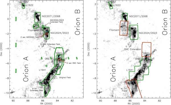
Figure 20. Distributions of the maximum change in magnitude for variable sources. In all cases, we chose sources where S > 2σS(photo). We show the maximum deviation in magnitude over the two to three epochs for all four IRAC bands, dividing the variable sources into stars with disks (upper row) and protostars (lower row).
Download figure:
Standard image High-resolution image
Table 7. Percentiles for Δm(λ)
| Wavelength | Evolutionary | Number | Δmag by Percentile | |||
|---|---|---|---|---|---|---|
| Band | Class | 25% | 50% | 75% | 10% | |
| 3.6 μm | Disks | 838 | 0.12 | 0.17 | 0.25 | 0.36 |
| 4.5 μm | Disks | 838 | 0.13 | 0.18 | 0.26 | 0.37 |
| 5.8 μm | Disks | 665 | 0.10 | 0.17 | 0.25 | 0.36 |
| 8 μm | Disks | 542 | 0.07 | 0.13 | 0.21 | 0.32 |
| 3.6 μm | Protostars | 167 | 0.16 | 0.24 | 0.38 | 0.53 |
| 4.5 μm | Protostars | 167 | 0.15 | 0.23 | 0.33 | 0.45 |
| 5.8 μm | Protostars | 151 | 0.12 | 0.20 | 0.31 | 0.44 |
| 8 μm | Protostars | 119 | 0.16 | 0.24 | 0.40 | 0.53 |
Download table as: ASCIITypeset image
4.3. Constraints on the Mechanism for Variability
We find evidence of variability for 50% of the YSOs with IR-excesses. The magnitude changes are approximately the same in all four IRAC bands and are typically on the order of 0.2 mag. Both the fraction of sources with variability and the changes in magnitude are largest for protostars. Since diskless objects do not exhibit similar variability, it is likely that the observed variability is due to the changes in the emission from the inner disk region where dust emits strongly in the IRAC bands. This emission is thought to originate primarily in the inner rim of the disk; at this inner rim the central stars heats the dust to the sublimation temperature of silicate grains. Dust within this radius will be sublimated, thus eliminating the primary source of opacity in the disk. Since the disk is vertically extended, the emission in the inner rim originates come from an "opacity wall" facing the central star. The infrared emission from the disk traced by the IRAC bands arises mainly in the rim, but it includes contributions from disk radii up to 1 AU, particularly in the 8 μm band (D'Alessio et al. 2006).
The variations in overall disk flux could be due to changes in the heating of the disk, fluctuations in its physical structure, or some combination of the two. The wavelength dependence of the variability, as measured by the slope of Δmλ versus Δ[4.5], and the timescale of the variations provide constraints on the mechanism for the infrared variability. A physical model for the variability must explain how material over the inner 1 AU could uniformly change its flux over the course of six months. Variations on timescales of less than one year could be due to fluctuations and rotating structures in the inner 1 AU of the disk where the dynamical timescale ranges from months to days with decreasing radius. These variations may result from a variety of reasons such as a rotating disk warp or magneto-rotational instability instabilities that launch dust out of the midplane (Turner et al. 2010). Previous observational studies have invoked scale height perturbations to the dust at the very inner edge of the disk to explain the wavelength dependence and timescale of the variability for evolved transition disks where the inner disk has been cleared. Scale height perturbations at the very inner edge of a disk result in a "seesaw" behavior for the infrared spectral energy distribution (SED), in which the short-wavelength flux increases while the long-wavelength flux decreases with the entire SED appearing to pivot at 8 μm (Flaherty et al. 2011; Espaillat et al. 2011). The observed variability could also result from changes in the heating of the inner disk by the central star. The disk is heated by both the intrinsic luminosity of the star and the accretion luminosity generated by gas funneled down onto the star. Changes in the heating of a disk could arise from fluctuations of the accretion rate onto the central star and the resultant change in accretion luminosity. The accretion luminosity is thought to be concentrated in accretion hot spots; the rotation of these hot spots may also result in variations in the heating of the portions of the inner disk most visible from the Earth (Bouvier & Bertout 1989; Morales-Calderón et al. 2009).
To examine how changes in the structure and heating of the inner disk would affect the observed magnitudes in the IRAC bands, we employ the CGPlus models (Chiang & Goldreich 1997; Dullemond et al. 2001). These models include a two-layer, flared disk with a puffed-up inner wall. While more complicated combinations of grain growth and settling are often needed to fit detailed SEDs, we can use these models to estimate the wavelength dependence due to changes in the disk and star. Our base model consists of a 0.5 M☉, 2 L☉, Teff = 3800 K star surrounded by a 0.01 M☉ disk that extends from the dust sublimation radius, defined as the point where Tdust = 1500 K, out to 100 AU. From these models, we can directly estimate magnitudes, and by varying different model parameters we can calculate the slope of Δmλ versus Δ[4.5] in the same manner as was done with the actual data. First, we consider variations due to a puffed-up inner rim by increasing the scale height of the dust and gas of the inner rim. In this case, we find slopes of 1.014, 0.96, and 0.60 for [3.6], [5.8], and [8.0], respectively (Table 8). While the radiative transfer in the shadowed region behind the inner rim is not fully understood, changing the scale height in this way produces a "seesaw" behavior similar to what has been observed in transition disks and thus serves as a useful approximation. The calculated slopes are inconsistent with the observations, suggesting that in the majority of the YSOs, the variability is not due to a change in the scale height of the inner disk rim. We next vary the radial location of the inner rim of the disk by lowering the temperature at which the disk becomes truncated. In this situation, we find slopes of 0.53, 1.468, and 1.499 which are also highly inconsistent with the data (Table 8). This implies that, unlike in the evolved disks, we are not observing a change in the structure of the dust at the very inner edge of the disk. We cannot rule out synchronized changes in the disk scale height over the entire inner 1 AU, which would affect all the IRAC bands equally; however, it is not clear what mechanism could alter the disk in this manner.
Table 8. Slope of Model Δmλ Variations
| Model | [3.6] | [5.8] | [8.0] |
|---|---|---|---|
| Observed | 0.865 ± 0.034 | 1.055 ± 0.036 | 1.273 ± 0.091 |
| Inner disk scale height | 1.014 | 0.96 | 0.60 |
| Inner disk radius | 0.53 | 1.468 | 1.499 |
| Vary star, not disk | 1.09 | 0.861 | 0.687 |
| Vary star and disk | 0.985 | 1.012 | 1.013 |
| Vary disk, not star | 0.922 | 1.053 | 1.124 |
Download table as: ASCIITypeset image
Next, we consider changing the stellar flux in the CGPlus models without varying the flux of the disk. This produces slopes of 1.09, 0.861, and 0.687 for [3.6], [5.8], and [8.0], respectively; these values show the decreasing dominance of the stellar photosphere with increasing wavelength. The lack of agreement with the observed slopes confirms the need for a change in the disk flux. If we vary the stellar luminosity while allowing the disk structure to respond to this change in the impinging flux, we find slopes of 0.985, 1.012, and 1.013. If we vary the disk heating without varying the infrared emission from the photosphere, which would be the case if the disk was heated by UV radiation from the accretion of gas onto the star, the resulting slopes of 0.922, 1.053, 1.124 provide the best match to the data (Table 8). In this case, the reduced slope at [3.6] is due to the significant contribution of the photosphere in that band. The thermal timescale of the upper layers of the disk that are responsible for the observed infrared emission are very short (Chiang & Goldreich 1997) and the disk will respond almost instantaneously to changes in the illumination. This suggests that we are observing a change in the overall flux level of the disk by an amount that is relatively constant with wavelength. Variable heating may come from rapid changes in the rate of accretion of gas onto the central stars; the accretion luminosity contributes significantly to the total luminosity of protostars and young stars with disks. Alternatively, Morales-Calderón et al. (2009) constructed models of the variable heating in a protostar due to a rotating accretion hot spot. In this case, the variability is not due to a change in total luminosity, but due to the region of the inner disk rim illuminated by the hot spot rotating in and out of view. These models also produce a wavelength dependence that is similar to what has been observed. We note that the Morales-Calderón et al. (2009) models which add a disk warp rotating in sync with the hot spot predicts a weaker variability at [8.0]; this is inconsistent with our observations.
We conclude that the time variable heating of an extended portion of the disk driven by rotating accretion hot spots or rapid accretion variations is the most likely explanation for the observed variations in the mid-IR magnitudes. This is in distinct contrast to transition disks for which structural perturbations of the puffed-up wall at the dust sublimation radius can explain the observed mid-IR variability (Flaherty et al. 2011; Espaillat et al. 2011). Hence, the mechanism for mid-IR variability may change as young stars objects and their disks evolve. A more definitive assessment of the origin of the variability will require coordinated observations designed to study the time dependence of mid-IR emission, stellar luminosity, and accretion (e.g., Flaherty et al. 2012).
5. SUMMARY
We present a survey of dusty YSOs identified in the Orion A and B clouds using the IRAC and MIPS instruments on board the Spitzer Space Telescope and the 2MASS point source catalog. This survey covered 8.8 deg2 of the Orion clouds in the four IRAC bandpasses and 16.4 deg2 with the MIPS instrument, with a combined total coverage of 8.8 deg2. In addition, eight reference fields covering 0.29 deg2 were observed with IRAC. In this paper, we present the catalog of point sources and YSOs, with the following results:
-
1.Within this field, 298,405 point sources are identified; a total of 34,176 are detected in a sufficient number of wave bands that they can be examined for infrared excesses. We characterize the completeness of the point source catalog as a function of magnitude in the four IRAC and one MIPS band. The completeness is spatially varying and is strongly dependent on the amount of nebulosity in a given field.
-
2.A total of 3479 dusty YSOs are identified by the presence of mid-infrared emission in excess of that expected for a reddened photosphere. This includes 2991 young stars with disks, 428 protostars, and 50 faint candidate protostars. In addition, another 10 sources detected only in the MIPS 24 μm band are candidate protostars. The identified dusty YSOs are found distributed throughout the Orion A and B clouds molecular clouds; a detailed analysis of the spatial distribution will be presented in a subsequent paper. We employed several criteria for rejecting contaminating galaxies; the residual contamination to the YSO sample from background galaxies is estimated to be 6.1 ± 3.1 per square degree. Using a Monte Carlo simulation of the background contamination, we estimate that an additional 13 sources may not be YSOs, but instead show YSO-like colors due to a blending with nebulosity and other point sources.
-
3.The YSOs were examined for variability using three epochs for the L1641 cloud and two epochs for the remainder of the survey. The dusty YSOs show a high degree of correlated variability in the 3.6 and 4.5 μm bands relative to pure photospheric sources without IR-excesses, with 50% of the dusty YSOs exhibiting significant variability. The median variability is 0.2 mag, with variations up to 1.76 mag detected. The protostars show both a higher incidence of variability and larger variations in their mid-IR magnitudes than young stars with disks. The variability is correlated in all four IRAC bands with the changes in the 5.8 and 8 μm bands approximately equal to those at 4.5 μm, and the 3.6 μm band showing somewhat weaker changes. Using models of the heating of an inner, puffed-up disk by a central source, we find that models that invoke changes in the heating of the inner disk best reproduce the observed variability. These changes may arise from fluctuations in the accretion rate or from rotating accretion hot spots.
This publication makes use of data products from the Two Micron All Sky Survey, which is a joint project of the University of Massachusetts and the Infrared Processing and Analysis. Center/California Institute of Technology, funded by the National Aeronautics and Space Administration and the National Science Foundation. This work is based in part on observations made with the Spitzer Space Telescope, which is operated by the Jet Propulsion Laboratory, California Institute of Technology under a contract with NASA. This work received support through that provided to the IRAC and MIPS instruments by NASA through contracts 960541 and 960785, respectively, issued by JPL. Support for this work was also provided by NASA through awards to STM and JLP issued by JPL/Caltech.
APPENDIX: MEASURING THE COMPLETENESS TO POINT SOURCES IN EACH WAVELENGTH BAND
To assess the completeness of the data, artificial stars were added to the ONC field in the four IRAC bands and the MIPS 24 μm bands. As described in Section 2, the Orion data exhibit spatially varying completeness primarily due to confusion with the bright and highly structured nebulosity detected in all wavelength bands. Instead of measuring the completeness for each position in the IRAC and MIPS maps, we determine completeness as a function of RMEDSQ, as defined in Section 2. To do this, we used the ONC field since this field shows the largest range in RMEDSQ values.
For the IRAC artificial stars, we used a PRF that was reconstructed from the observations of an IRAC standard star.13 To account for the rotation of the spacecraft during the two epochs of the observation, the artificial PRF was the sum of two rotated PRFs. The artificial star analysis was done separately for "faint," "bright," and "ultra-bright" stars. The input magnitudes of the faint stars were distributed in 0.5 mag increments between 12.5 and 16.5 mag for the 3.6 and 4.5 μm bands, and between 10.5 and 14.5 mag for the 5.8 and 8 μm bands. Bright stars were added in 0.5 mag increments between 8 and 12 mag for the 3.6 and 4.5 μm bands, and between 6 and 10 mag for the 5.8 and 8 μm bands. Finally, the ultra-bright stars covered 3.5–7.5 mag in 0.5 mag increments for the 3.6 and 4.5 μm bands and 1.5–5.5 mag in 0.5 mag increments for the 5.8 and 8 μm bands. In all three cases, the stars were distributed in a rectangular grid in which each added star was separated by 125 from the adjacent artificial stars.
The added stars were then recovered with PhotVis using automated source detection; any source within 15 of the input position, within 0.25 mag of the input source magnitude, and with uncertainties within the limits set for YSO identification (0.1 mag for the 3.6 and 4.5 μm bands and 0.15 mag for the 5.8 and 8 μm bands) was considered recovered. The PhotVis object detection parameters were the same as those used for the point source catalog. The recovered faint stars were binned by their log(RMEDSQ) values using a bin of 0.5. The reason for the logarithmic binning is that increasingly bright nebulous regions cover progressively smaller portions of the image; a logarithmic binning thus provides better statistics for regions where RMEDSQ > 1000. We then calculated the fraction of recovered stars (nrec) to added stars (nadd) using the equation f = nrec/nadd. The fractions as a function of input magnitude and log(RMEDSQ) are shown for the IRAC bands in Figure 3.
For the purpose of the correction, it is of value to obtain for each magnitude a continuous curve parameterized by the RMEDSQ. For each input magnitude of the artificial stars, we fit a function to the fraction of recovered stars versus log(RMEDSQ). We fit the equation

where a and b are the value of RMEDSQ at which the completeness declines to 0.5 and the width of the decline, respectively. This equation has desirable features of having a fraction approaching one for small values of log(RMEDSQ) and a fraction approaching zero for high values of log(RMEDSQ). When fitting the data, we adopted an uncertainty

which is the uncertainty from Bolte (1989) with a noise floor added to both high and low values of f. The noise floors were set by using trial and error to find values of σf for which the fit would converge. The resulting fits are shown in Figure 3. The values of a and b for the selected magnitudes are shown in Table 9.
Table 9. Fits to Single-band Completeness Curves
| Mag | 3.6 μm | 4.5 μm | Mag | 5.8 μm | 8 μm | Mag | 24 μm | |||||
|---|---|---|---|---|---|---|---|---|---|---|---|---|
| aa | ba | aa | ba | aa | ba | aa | ba | aa | ba | |||
| 8.0 | 4.37 | 0.30 | 3.84 | 0.15 | 6.0 | 4.01 | 0.22 | 4.14 | 0.25 | 2.00 | 4.09 | 0.50 |
| 8.5 | 4.06 | 0.27 | 3.75 | 0.17 | 6.5 | 3.83 | 0.32 | 3.94 | 0.26 | 2.50 | 3.93 | 0.50 |
| 9.0 | 3.74 | 0.24 | 3.49 | 0.28 | 7.0 | 3.61 | 0.26 | 3.72 | 0.26 | 3.00 | 3.72 | 0.53 |
| 9.5 | 3.65 | 0.30 | 3.28 | 0.23 | 7.5 | 3.44 | 0.30 | 3.54 | 0.26 | 3.50 | 3.34 | 0.44 |
| 10.0 | 3.41 | 0.28 | 3.04 | 0.18 | 8.0 | 3.19 | 0.27 | 3.34 | 0.28 | 4.00 | 3.15 | 0.40 |
| 10.5 | 3.20 | 0.30 | 2.87 | 0.23 | 8.5 | 3.01 | 0.26 | 3.12 | 0.23 | 4.50 | 2.94 | 0.39 |
| 11.0 | 3.01 | 0.25 | 2.69 | 0.23 | 9.0 | 2.82 | 0.28 | 2.96 | 0.25 | 5.00 | 2.78 | 0.41 |
| 11.5 | 2.81 | 0.28 | 2.48 | 0.23 | 9.5 | 2.59 | 0.24 | 2.75 | 0.28 | 5.50 | 2.63 | 0.46 |
| 12.0 | 2.60 | 0.27 | 2.25 | 0.22 | 10.0 | 2.40 | 0.27 | 2.54 | 0.23 | 6.00 | 2.42 | 0.44 |
| 12.5 | 2.41 | 0.28 | 2.04 | 0.21 | 10.5 | 2.19 | 0.24 | 2.31 | 0.28 | 6.50 | 2.21 | 0.43 |
| 13.0 | 2.19 | 0.27 | 1.84 | 0.21 | 11.0 | 1.99 | 0.26 | 2.08 | 0.26 | 7.00 | 1.98 | 0.43 |
| 13.5 | 1.99 | 0.25 | 1.65 | 0.21 | 11.5 | 1.79 | 0.28 | 1.87 | 0.28 | 7.50 | 1.80 | 0.44 |
| 14.0 | 1.81 | 0.29 | 1.44 | 0.20 | 12.0 | 1.58 | 0.24 | 1.65 | 0.25 | 8.00 | 1.58 | 0.46 |
| 14.5 | 1.58 | 0.24 | 1.23 | 0.20 | 12.5 | 1.37 | 0.27 | 1.44 | 0.26 | 8.50 | 1.32 | 0.44 |
| 15.0 | 1.37 | 0.27 | 1.00 | 0.20 | 13.0 | 1.13 | 0.25 | 1.20 | 0.25 | 9.00 | 0.89 | 0.54 |
| 15.5 | 1.13 | 0.26 | 0.76 | 0.20 | 13.5 | 0.89 | 0.27 | 0.96 | 0.25 | 9.50 | 0.21 | 0.07 |
| 16.0 | 0.89 | 0.26b | 0.49 | 0.19 | 14.0 | 0.64 | 0.24 | 0.65 | 0.26 | 10.00 | 0.16 | 0.05 |
| 16.5 | 0.64 | 0.24c | 0.21 | 0.15 | 14.5 | ... | ... | ... | ... | ... | ... | ... |
Notes. aUncertainties for a and b are ⩽0.01 unless noted. bUncertainty is 0.11. cUncertainty is 0.15.
Download table as: ASCIITypeset image
The MIPS 24 μm completeness was assessed in a similar way. A grid of point sources were added to the images; the point source was generated by STinyTim for a 50 K source. This was done with two iterations: one for faint stars with magnitudes ranging from 6.5 to 10.5 mag in increments of 0.5 mag and the other for bright stars with magnitudes ranging from 2 to 6 mag in increments of 0.5 mag. The stars were separated by 12.5 pixels. Point sources detected by PhotVis with positions and magnitude within 15 of the input position, 0.25 mag of the input magnitude and with an uncertainty ⩽0.25 mag were considered recovered. The PhotVis object detection parameters were the same as used for the point source catalog and the magnitudes were determined using aperture photometry using the aperture radius, sky annulus, and calibration described in Section 2.5. The number of recovered and added stars were binned in intervals of log(RMEDSQ), and the resulting fraction was fit repeating the steps for the IRAC data (Figure 4). The values of a and b for the MIPS data are shown in Table 9.
Footnotes
-
11
-
12
-
13