


ABSTRACT
We investigate the intrinsic stellar populations (estimated total numbers of OB and pre-main-sequence stars down to 0.1  ) that are present in 17 massive star-forming regions (MSFRs) surveyed by the MYStIX project. The study is based on the catalog of >31,000 MYStIX Probable Complex Members with both disk-bearing and disk-free populations, compensating for extinction, nebulosity, and crowding effects. Correction for observational sensitivities is made using the X-ray luminosity function and the near-infrared initial mass function—a correction that is often not made by infrared surveys of young stars. The resulting maps of the projected structure of the young stellar populations, in units of intrinsic stellar surface density, allow direct comparison between different regions. Several regions have multiple dense clumps, similar in size and density to the Orion Nebula Cluster. The highest projected density of ∼34,000 stars pc−2 is found in the core of the RCW 38 cluster. Histograms of surface density show different ranges of values in different regions, supporting the conclusion of Bressert et al. that no universal surface-density threshold can distinguish between clustered and distributed star formation. However, a large component of the young stellar population of MSFRs resides in dense environments of 200–10,000 stars pc−2 (including within the nearby Orion molecular clouds), and we find that there is no evidence for the B10 conclusion that such dense regions form an extreme "tail" of the distribution. Tables of intrinsic populations for these regions are used in our companion study of young cluster properties and evolution.
Export citation and abstract BibTeX RIS
1. INTRODUCTION
The Milky Way Galaxy is a critical part in the universe for studying star formation. Only here can the populations of low-mass stars—making up the vast majority of stars—be resolved and the full spatial structure of young stellar clustering and molecular clouds be analyzed, revealing detailed information about how star formation progresses within a region. Most stars, including the Sun (Gounelle & Meynet 2012; Dukes & Krumholz 2012), are born in clusters with OB-type stars, so it is important to study the massive star-forming regions (MSFRs) in the solar neighborhood. The young stellar clusters in these regions can be precursors to open clusters, but most of their stars become gravitationally unbound due to gas expulsion, so an understanding the star-formation histories and early cluster dynamics in these regions provides clues about how bound clusters and field stars are produced (e.g., Goodwin & Bastian 2006; Pfalzner 2011; Kruijssen et al. 2012; Banerjee & Kroupa 2014).
Historically, studies of massive Galactic star-forming regions have been hindered by difficulties inherent to Galactic Plane astronomy; in particular, field stars greatly outnumber members of the star-forming region in optical or infrared (IR) images (e.g., King et al. 2013; Kuhn et al. 2013b). X-ray surveys readily detect star-forming region members due to the high X-ray luminosities from strong magnetic activity of pre-main-sequence stars ( ; Preibisch et al. 2005a), and these surveys are not strongly effected by nebulosity, obscuration, or crowding. Excess IR emission from disk-bearing young stars has proven to be another useful method of establishing membership, but IR-only surveys will miss the large populations of members without dusty protoplanetary disks and such studies rarely account for observational sensitivities in determining intrinsic stellar populations, as we attempt to do in this paper. The combination of X-ray selected stars and IR-excess selected stars can provide better samples of stars in MSFRs than either method alone (Feigelson et al. 2013; Townsley et al. 2011). Thus, the analysis of empirical distributions of inferred stellar mass and X-ray luminosities from the combined samples can be used to estimate total populations (e.g., Getman et al. 2012, and references therein).
The Massive Young Star-Forming Complex Study in IR and X-ray (MYStIX; Feigelson et al. 2013) examines 20 nearby MSFRs using a combination of archival Chandra X-ray imaging, 2MASS+UKIDSS near-IR (NIR), and Spitzer mid-IR (MIR) survey data. The catalogs of young stars include both high-mass and low-mass stars, and disk-bearing and disk-free stars (Broos et al. 2013). We use this sample of stars to study the intrinsic populations of young stars across 17 of the MYStIX MSFRs.
The present study is closely based on the constructions of the MYStIX Probable Complex Members catalog (MPCM; Broos et al. 2013) and the statistical segregation of MPCMs into ∼140 subclusters by Kuhn et al. (2014, Paper I). Our principal objective here is to overcome sensitivity limitations of the MPCM catalog for each MYStIX MSFR in order to normalize the observed stellar distributions to intrinsic stellar distributions. We obtain two quantities of interest: the total intrinsic stellar population and the stellar surface densities in each MYStIX subcluster. The total populations are important inputs into a multivariate analysis of young cluster properties in our forthcoming study (Kuhn et al. 2014, Paper III). The stellar surface densities address long-standing issues about typical environments in which stars form.
1.1. Thresholds for Clustered Star Formation
The statistical relationships that traditionally underlay our understandings of star-formation processes have been scale-free relationships like the Salpeter (1955) stellar initial mass function (IMF) and the Kennicutt–Schmidt law relating global galactic star-formation rate to interstellar material (Schmidt 1959; Kennicutt & Evans 2012). Nevertheless, important preferred scales for star formation were later found. The power-law IMF for high stellar masses peaks around 0.2–0.3  and declines for lower mass stars (Chabrier 2003). And, in the Galactic neighborhood, a threshold for star formation was found at
  magnitudes dust absorption (
![$\approx n[{{H}_{2}}]\sim 3\times {{10}^{4}}$](https://content.cld.iop.org/journals/0004-637X/802/1/60/revision1/apj508569ieqn5.gif) cm−3) associated with Galactic disk stability (Johnson et al. 2004; Lada 2010; Martin & Kennicutt 2001; Schaye 2004; Leroy et al. 2008), although this rule is not applicable within the inner 0.5 kpc of the Galaxy where star formation is comparatively suppressed (Longmore et al. 2013).
cm−3) associated with Galactic disk stability (Johnson et al. 2004; Lada 2010; Martin & Kennicutt 2001; Schaye 2004; Leroy et al. 2008), although this rule is not applicable within the inner 0.5 kpc of the Galaxy where star formation is comparatively suppressed (Longmore et al. 2013).
The surface density of stellar populations in star-forming regions, in units of stars per square parsec, has been a property of interest for the field of star-cluster formation (e.g., Carpenter 2000; Lada & Lada 2003; Allen et al. 2007; Jørgensen et al. 2008; Gutermuth et al. 2009). The surface densities of young stars can also have astrophysical implications, such as tidal truncation of protoplanetary disks (Pfalzner et al. 2005), binary star distributions (Bate 2009a; Moeckel & Clarke 2011), or the survival of clusters after molecular cloud dispersal (Kruijssen 2012). (Bressert et al. 2010, henceforth B10) have recently examined the shape of the distribution of stellar surface densities in star-forming regions. They use samples of disk/envelope-bearing stars identified through IR excess in regions within 0.5 kpc of the Sun, including the Gould Belt (Allen et al. 2006), the Orion A and B molecular clouds (Megeath et al. 2012), the Taurus molecular cloud (Rebull et al. 2010), and the regions from the cores-to-disks (c2d; Evans et al. 2003) project—thus their sample is dominated by low-mass young stellar object (YSO) environments. B10 argue that if "clustered" star formation and "distributed" star formation were two distinct star-formation processes, then "clustered" and "distributed" populations should appear as distinct modes in the surface-density distribution (cf. Gieles et al. 2012; Pfalzner et al. 2012), and that such a scenario could be tested by searching for a "scale" of star formation separating these two modes. Such a kink in the surface-density distribution has been used in some investigations of the structure of young stellar clusters, for example by Gutermuth et al. (2009), to separate distinct clusters of stars in star-forming regions. Given that B10 find a smooth distributions of surface density from their data, which they report is adequately fit by a log-normal distribution with a peak at 22 stars pc−2, they conclude that no such "scale" exists, at least for low-mass YSO environments present in the solar neighborhood.
Nevertheless, the log-normal distribution from B10 is not scale free, but instead a peak at 22 stars pc−2 and width of 0.85 dex suggests a density distribution weighted toward low-density environments. If this result is a general characteristic of most star formation in the Galaxy, rather than just the nearby regions investigated by B10, it would have implications for theories of star formation as numerous researchers have discussed. For example, Parmentier & Pfalzner (2013) find that their models of local-density-driven star formation from a single molecular clump could produce the 22 stars pc−2 scale from B10. King et al. (2012) suggest that surface densities significantly greater than 22 stars pc−2 could indicate that a cluster has undergone a "cool collapse phase." Kruijssen et al. (2012) present a model in which the low fraction of star formation that results in bound clusters is, in part, a result of a density spectrum weighted toward low surface densities. Parker et al. (2011) notes that dynamical processing of primordial binaries by clusters depends on whether most stars form in low density regions as suggested by B10, or whether higher density clusters are more common. And, de Juan Ovelar et al. (2012) investigate the threshold densities in star-forming regions where stellar interactions affect habitable planet formation—and the fraction of the stars born in environments above their 3 × 10³ stars pc−2 threshold would depend on whether high-density regions are just a tail of the B10 log-normal or a different mode not seen in the B10 sample. B10 support this interpretation of the empirical results from their sample stating, "only a small fraction (<26%) of stars form in dense clusters where their formation and/or evolution is expected to be influenced by their surroundings."
It is important to investigate whether these results continue to hold for more MSFRs (those regions containing O-type stars). Nearly 70% of B10's sample comes from the Orion giant molecular clouds, which do contain O-type stars, but they note that the IR-excess methods used are ineffective at identifying young stars in the presence of nebulosity and crowding in this complex. Their other star-forming regions are lower mass. Given that studies of the mass function for star-forming regions favor the birth of stars in more massive complexes, investigation of these complexes in a way that is more effective at probing the densest regions could be helpful for determining the validity of B10's suggestion that clustered stars ( stars pc−2) exist in the tail of the surface-density distribution, rather than being a dominant component. Nevertheless, a definitive study of surface-density distributions for star formation would require the construction of an unbiased survey of all star-forming environments. MYStIX neither includes the most massive star-forming environments in the Galaxy (such as W 43, Wd 1, NGC 3603, or the Arches Cluster) nor includes large angular area studies of diffuse molecular clouds necessary to capture the lowest surface density environments.
1.2. MYStIX
The MYStIX survey (Feigelson et al. 2013) differs from many previous studies in that it focuses on relatively MSFRs lying in nearby Galactic spiral arms, and supplements samples of IR-excess young stars with X-ray selected young stars and spectroscopically identified OB stars.
MYStIX is a survey of 20 of the nearest ( kpc) MSFRs that have been observed with NASA's Chandra X-ray Observatory, the Spitzer Space Telescope, and the United Kingdom Infra-Red Telescope (UKIRT) or the Two Micron All Sky Survey (2MASS; Skrutskie et al. 2006). The MYStIX regions include the Orion Nebula, the Flame Nebula, W40, RCW 36, NGC 2264, the Rosette Nebula, the Lagoon Nebula, NGC 2362, DR 21, RCW 38, NGC 6334, NGC 6357, the Eagle Nebula, M17, W 3, W 4, the Carina Nebula, the Trifid Nebula, NGC 3576, and NGC 1893, from which a sample of 31,784 MYStIX Probable Complex Members (MPCMs; Broos et al. 2013) is obtained. The MPCM catalog thus consists of young stars that are X-ray selected, IR excess selected, or OB stars from the literature. MYStIX provides the cleanest and largest lists of young stars for most of the 20 regions included in the study, so these catalogs should be scientifically useful for different purposes. One of the requirements of the MYStIX project was to use sensitive and homogeneous data analysis procedures for all 20 regions to facilitate inter-comparisons between regions. Special procedures had to be developed to deal with challenges working in the Galactic Plane, as described in the MYStIX technical-catalog papers: Kuhn et al. (2013a), Townsley et al. (2014), King et al. (2013), Kuhn et al. (2013b), Naylor et al. (2013), Povich et al. (2013), and Broos et al. (2013).
The spatial distributions of MPCMs in 17 of the MYStIX MSFRs are investigated in Kuhn et al. (2014, henceforth Paper I) and in this work. Three regions are omitted, NGC 3576, W 3, and W 4, because they lack JHK UKIRT photometry and have a low match rate between X-ray sources and sources from the 2MASS catalog. We use a subset of the MPCM sources (∼17,000 stars) produced after X-ray selected MPCMs are pruned to a uniform X-ray sensitivity within each region (Paper I). This eliminates artificial surface density gradients associated with differing X-ray exposure times in Chandra mosaics and the sensitivity variations within each Chandra field due to telescope coma and vignetting, the "egg-crate effect" (Townsley et al. 2011). To prune a region, we remove sources with X-ray photon fluxes (log_PhotonFlux_t; Broos et al. 2013) that are lower than the completeness limits provided in Table 1 of Paper I.
Table 1. XLF Properties of MSFRs
| Region |  |
Ntot |  |
 |
 |
|---|---|---|---|---|---|
| (stars) | (stars) | (stars) | (stars) | ||
| (1) | (2) | (3) | (4) | (5) | (6) |
| Orion | −0.9 | 2600 | 700 | 1200 | 720 |
| Flame | −1.0 | 800 | 55 | 250 | 500 |
| W40 | −1.1 | 520 | 0 | 250 | 270 |
| RCW 36 | −0.8 | 550 | 0 | 230 | 320 |
| NGC 2264 | −1.0 | 1900 | 1100 | 230 | 570 |
| Rosette | −1.3 | 2500 | 840 | 1000 | 610 |
| Lagoon | −1.1 | 3800 | 2000 | 870 | 930 |
| NGC 2362 | −1.1 | 600 | 570 | 30 | 0 |
| DR 21 | −1.0 | 2900 | 50 | 550 | 2253 |
| RCW 38 | −1.3 | 9900 | 70 | 1900 | 8000 |
| NGC 6334 | −1.2 | 9400 | 180 | 2900 | 6200 |
| NGC 6357 | −1.2 | 12000 | 440 | 7400 | 3700 |
| Eagle | −1.3 | 8100 | 1300 | 4300 | 2500 |
| M17 | −1.3 | 16000 | 170 | 5400 | 11000 |
| Carina | −1.5 | 34000 | 9500 | 17000 | 7000 |
| Trifid | −1.0 | 3100 | 1500 | 1100 | 470 |
| NGC 1893 | −1.5 | 4600 | 1700 | 2400 | 590 |
Note. Column 1: name of MYStIX MSFR. Column 2: power-law index ( ) for the portion of the XLF tail shown in Figure 2 (uncertainties are ±0.1). Column 3: inferred intrinsic total population. Columns 4–6: inferred intrinsic numbers of stars with
  keV,
keV,  keV, and
  keV, respectively. (Due to rounding, the sum of Columns 4, 5, and 6 is not always equal to Column 3.)
Download table as: ASCIITypeset image
Nevertheless the resulting observed surface densities, used by the analysis in Paper I, do not contain the entire intrinsic population, differ in sensitivity from MSFR to MSFR, and are affected by spatially variable NH absorption and MIR sensitivity. As pre-main-sequence (PMS) X-ray luminosities strongly scale with stellar mass (Telleschi et al. 2007), inconsistent X-ray sensitivities due to differing Chandra exposure times and MSFR distances lead to different samplings of the cluster IMFs. We overcome these selection effects calibrating the observed X-ray luminosity function (XLF) and IMF distributions to the Orion Nebula Cluster (ONC) that serves as a template for young cluster populations, rather than attempting to model instrumental and observational effects.
The organization of this paper (Paper II) is as follows. We analyze the IMF and XLF to infer intrinsic populations from observed young stellar populations (Section 2). We derive intrinsic stellar surface density maps from these populations (Section 3), and investigate surface density distributions (Sections 4 and 5). The MYStIX sample of star-forming regions are typically richer than those in the sample studied by B10. The MYStIX MSFRs exhibit a large diversity in their surface density distributions (ranging from ∼10 to ∼30,000 stars pc−2), neither showing a tendency to follow a universal surface density distribution nor showing a convincing peak at some characteristic surface density. These results are discussed in Sections 4 and 5 and summarized in the conclusion (Section 6).
2. STELLAR POPULATIONS
The completeness limits and detection fractions4 of the MPCM samples vary from region to region, due to differences in distance, obscuration, and X-ray and IR observation exposures. Extrapolations of the total numbers of stars in a region, which we infer empirically from observed MPCM samples based on comparisons with the ONC, are necessary for comparison of intrinsic properties of stellar populations in different star-forming regions.
2.1. X-ray Luminosity Functions
Young stars in the Chandra Orion Ultradeep Project (COUP; Getman et al. 2005b) had large numbers of X-ray counts, allowing X-ray luminosities ( ; total 0.5–8.0 keV band and absorption corrected) to be obtained by parametric modeling of the X-ray spectrum using the XSPEC code (Arnaud 1996). As the MYStIX stars are mostly too faint for this procedure, X-ray luminosities for other MPCMs were computed using non-parametric calibrations for PMS stars (XPHOT; Getman et al. 2010) by Kuhn et al. (2013a), Townsley et al. (2014), Broos et al. (2011), and Kuhn et al. (2010).
The probability distribution of  , called the XLF, is associated with the IMF due to the statistical link between X-ray luminosity and stellar mass M (e.g., Feigelson et al. 1993; Preibisch et al. 2005a; Telleschi et al. 2007). The assumption of a "universal XLF" (Feigelson & Getman 2005) has been used to estimate total populations in young stellar clusters, including Cep B (Getman et al. 2006), M17 (Broos et al. 2007), NGC 6357 (Wang et al. 2007), Rosette (Wang et al. 2008, 2009, 2010), W40 (Kuhn et al. 2010), Trumpler 15 (Wang et al. 2011), Trumpler 16 (Wolk et al. 2011), Sh 2–254/255/256/257/258 (Mucciarelli et al. 2011), NGC 1893 (Caramazza et al. 2012), and IC 1396 (Getman et al. 2012). During PMS stellar evolution, there is a weak relation between X-ray luminosity and age (e.g., Preibisch & Feigelson 2005; Pandey et al. 2014); however,
  does not rapidly decline during the first 5 Myr, unlike the rapid decrease in bolometric luminosity Lbol during PMS evolution along the Hayashi track. Instead,
  appears to be the fundamental relationship rather than
  (Getman et al. 2014b). Thus, X-ray luminosity evolution appears to have little effect on the shape of the PMS XLF (e.g., Bhatt et al. 2013).
Following these previous studies, we use a sample of stars from COUP to approximate the probability distribution of the universal XLF. The COUP study contains a sample of 839 lightly absorbed stars (Feigelson et al. 2005), which are identified as the members of the ONC, while the more highly absorbed stars are identified as being embedded in the Orion Molecular Cloud (OMC) behind the ONC. These lightly obscured COUP stars are complete down to a mass of 0.1–0.2  (with partial coverage into the proto–brown-dwarf regime; Preibisch et al. 2005b) and show an XLF shape characterized by a falling distribution at high luminosities with a break to an approximately flat distribution at luminosities below
  erg s−1. Henceforth, we label this distribution the COUP XLF. The tail with X-ray luminosities greater than this turnover can be fit with a power-law (Pareto) distribution of slope α, with a minimum variance unbiased estimator
  and variance
  given by the equations

where xm is the X-ray luminosity of the turnover point and xi is the X-ray luminosity of the ith source in a sample of n sources in the distribution tail (Johnson et al. 1994). Thus,  with n = 61, while the distribution is roughly flat in logarithmic bins below the turnover point. Mucciarelli et al. (2011) have also found similar
  Pareto distributions for the ONC and the Sh 2-254–258 regions.
The  distributions for the MYStIX regions can be compared to the empirical distribution function (EDF) of 839 lightly absorbed COUP sources to further investigate the universality of the XLF shape. For example, Wang et al. (2008, their Figure 9(b)) shows that the XLF cumulative distributions in the Rosette star-forming region agree with the COUP XLF above the X-ray luminosity completeness limit for the Rosette sample. For this analysis it is necessary to be cautious about how completeness limits are treated because differential absorption can change the apparent shape of the XLF if the sample of highly absorbed sources is incomplete. For example, a sample of sources that are more deeply embedded will have a higher mean luminosity than a sample of sources from the same observation that are unabsorbed, which could lead to a flattening of the power-law of the combined distribution.
In Figure 1, we show the COUP EDF running from unity at very low luminosities ( erg s−1) to zero for the most luminous PMS star in the Orion Nebula field. Note that spectroscopically identified OB stars have been removed from both the COUP XLF and from MYStIX samples considered here because MYStIX regions can differ widely in their massive stellar subpopulations. The
  EDFs for the other regions are shown below, with arbitrary vertical spacings. Only the portion of the XLF where the sample is complete is shown. (The completeness limit for the full sample is set to the completeness limit for the most heavily obscured subpopulation in the region.) In general there is excellent agreement between the shapes of the different lines. Some curvature can be seen in the COUP XLF between
  erg s−1 and
  erg s−1, which is also reflected in the shapes of the XLFs for other regions. The nearest regions tend to probe a lower-luminosity section of the XLF, while the more distant regions tend to probe a higher-luminosity section of the XLF. Due to the XLF curvature, the XLF shape appears less steep for nearer regions and steeper for more distant regions. Table 1 (Column 2) gives the power-law indices5 (for the full sample) calculated over the regions shown in Figure 1. This confirms the trend in which more distant regions have steeper slopes—not because of differences in intrinsic XLF shape, but due to differences in the available portion of the XLF.

Figure 1. The EDF of X-ray luminosities, Lt,c for the 839 lightly obscured, low-mass stars from COUP (complete down to 0.1–0.2  ) is shown by the thick gray line. The black lines, from top to bottom, are the X-ray luminosity EDFs for the other MYStIX regions. Vertical shifts of 0.3 units are used to separate the different lines for visual clarity. Lines end at the completeness limit for the full sample (i.e., the completeness limit for the most heavily obscured subpopulation in the region).
Download figure:
Standard image High-resolution image2.1.1. Intrinsic Numbers of Stars
If we accept the assumption of a "universal XLF" with the COUP sample serving as a template, the total stellar population of a star-forming region may be extrapolated from the missing stars at low luminosities where the region's observed XLF has dropped to zero due to incompleteness, but where the existence of these stars may be inferred from the universal XLF shape. To perform this calculation, the COUP XLF histogram is scaled so that it matches the observed XLF in the section of the XLF where the observed sample is complete. The completeness limit for the full sample of young stars will be the completeness limit for the most absorbed subpopulation of stars in the region. However, few of the most deeply embedded protostars may be observed, so this population will be poorly characterized, and the inferred total populations may be considered lower limits that do not necessarily account for all undetected, embedded stars.
If we further assume that X-ray absorptions from the molecular cloud are independent of the intrinsic stellar X-ray luminosities, we can estimate the intrinsic numbers of stars with different amounts of absorption in the star-forming region—this is useful because it allows us to compare total populations in more extinguished parts of a star forming region to total populations in less extinguished areas. Using this assumption, any subset of stars selected by X-ray absorption will be drawn independently from the "universal XLF" and therefore have the same XLF shapes—allowing us to perform the XLF population analysis described above on the subset. This assumption may not be entirely true; for example, mass segregation may cause more X-ray luminous stars to lie preferentially in the center of a cluster where absorptions are often higher. There is also weak evidence for a factor of ∼2 systematic increase in X-ray luminosity from the younger Class I to the older Classes II/III systems (Prisinzano et al. 2008). Nevertheless, the absorption stratified MYStIX XLFs all show consistency with the COUP XLF, indicating that these are not major effects.
Interstellar medium absorption of MPCMs may be evaluated using  color indices or X-ray Median Energy (ME; Getman et al. 2010) indicators, both of which increase as absorbing columns increase (Getman et al. 2014b). The spread in absorptions for subclusters of stars is provided in Paper I (their Figure 8), which shows the median
  and ME for clusters of young stars in the MYStIX regions. There is a clump of data points with
  keV (the unembedded population), while the absorbed population ranges over
  keV. The bulk of the absorbed groups of stars are moderately absorbed, with
  keV, and tend to have physical properties similar to the unabsorbed clusters. In contrast, the most absorbed groups of stars are much more compact (
 pc) and tend to be centered on dense molecular filaments or clumps (Getman et al. 2014b).
We choose to stratify the MYStIX MPCM stars into three absorption strata using ME divisions at 1.5 and 2.5 keV. This captures different aspects of the spatial structure of the stars: roughly, the population of stars outside the molecular cloud, the population within the molecular cloud, and the population associated with dense molecular filaments and cores. Figure 2 shows the observed XLF histograms for these three subpopulations in NGC 6357 (black lines): the  keV sources (left), the
  keV sources (center), and the
  kev sources (right). The completeness limits in this region vary from
  , to
, to  , to
, to  , for these three strata, respectively. The template COUP XLF (gray lines) is scaled to these three populations, using a vertical shift that minimizes the area between the two EDFs in the range where the XLF is approximately complete. The XLFs of all three strata show agreement between the shape of the sample XLF and the COUP XLF. The intrinsic number of stars in each absorption stratum can be estimated by integrating the number of stars under the scaled universal XLF curve, i.e., the gray COUP line. Thus, the inferred intrinsic population in NGC 6357 is ∼440 lightly obscured stars, ∼7400 moderately obscured stars, and ∼3700 highly obscured stars.6 Similar plots of stratified XLFs are provided for the other 16 regions as a figure set in the electronic version of the article.

Figure 2.
The XLF for NGC 6357 X-ray selected MPCMs with (left panel)  keV, (center)
  keV, and (right)
  keV. Stars with known spectral types earlier than B3 are not included. The COUP XLF of 839 lightly absorbed stars is scaled to these populations. Completeness limits for the three absorption strata are indicate by the vertical dashed line. (The complete figure set (17 images) is available.)
Download figure:
Standard image High-resolution imageAs expected, for every region, the more highly absorbed strata have a higher  completeness limit than the less absorbed strata. Generally, there is good agreement with shape of the COUP XLF; however, in most cases the sample becomes incomplete before reaching the turnover point at
  erg s−1 in the XLF. The Flame Nebula is one of the few cases where the completeness limit is less luminous than the XLF turnover point in the lightly and moderately absorbed strata, so the "flat" portions of the XLFs can be compared—the figure indicates that the XLFs are consistent. There is also indication of this turnover in the lightly absorbed stratum for NGC 2264.
The extrapolated intrinsic stellar populations for each stratum in each region are provided in Table 1. These values are combined to produce estimates of the total intrinsic populations for each star-forming region (Column 3). These values of Ntot are the principal empirical results of this study. Effects of distance and observational sensitivity should be approximately corrected by this analysis, but inferred total populations for more distant, less complete regions will be less precise and may be affected by additional systematics. To investigate these effects, we simulate the X-ray sensitivity for the Orion Nebula region if it were at the distance of the Carina Nebula (∼2.3 kpc) with the pruned X-ray sensitivity ( ) for the Chandra Carina Complex Project (CCCP; Townsley et al. 2011). Getman et al. (2005a, their Table 3) report 21 close doubles with <2'' separations in COUP, which would be indistinguishable at the distance of Carina. For this test, we combine their X-ray luminosities into a single source for the purpose of X-ray sensitivity limits and XLF analysis. From the 120 X-ray sources in this reduced-sensitivity Orion sample (out of 1216 original X-ray sources), we infer a total of ∼2000 stars rather than ∼2600 stars. Thus our Ntot values may underestimate the true populations by up to ∼30%, with most of the missing stars from the highly obscured ME stratum. Effects of distance and observational sensitivity are mentioned in Sections 3 and 4.
2.1.2. Detection Fraction for X-ray Selected MPCMs
The MPCM X-ray detection fraction,  , can be used as a correction factor to convert observed surface densities of young stars into intrinsic surface densities. However, dividing the surface density of a region by a single detection fraction does not account for spatial variation in sensitivity. The statistical sample of X-ray selected young stars provided in Paper I, is a pruned subset of the MPCMs to which a uniform photon-flux limit is applied to correct for observational sensitivity effects, including Chandra telescope vignetting, variation in point-spread function, and differing net exposure times in a mosaicked field. However, their samples do not control for differing luminosity completeness limits due to variable extinction.
An improved estimate of stellar surface densities can be made using the absorption-stratified samples from Section 2.1.1. Each ME stratum has a narrower range of absorptions than the full sample, so the spatial variation in sensitivity within these samples will be lower than for the full sample. The sources in each stratum are adaptively smoothed (described below) to produce surface density maps, and the detection fraction for each stratum given by the XLF analysis.
The spatially dependent detection fractions for the full Paper I X-ray selected samples are computed using the equation,

where fi is the detection fraction of the ith stratum and  is the adaptively smoothed observed surface density of that stratum. Detection fraction tends to be roughly constant across the fields of view, with dips found where molecular clouds and cores are located. But, detection fraction varies strongly between regions, so it is essential that scientific comparison between regions be based on the intrinsic young stellar surface densities rather than observed MPCM surface densities.7
Figure 3 shows detection fraction maps for the Carina, Eagle, and NGC 6334 fields of view. The larger distance and shorter Chandra exposure times for the Carina Nebula compared to the Eagle Nebula result in a lower overall detection fraction for Carina compared to Eagle. In the Eagle Nebula, the bubble around the main NGC 6611 cluster results in a relatively high detection fraction, while the embedded subclusters to the northeast have lower detection fractions. A molecular filament passes through NGC 6334 from northeast to southwest, producing a notable trough in the detection fraction map of this region. Overall, detection fractions for MYStIX MSFRs range between 1–60%.

Figure 3. The inferred fractional completeness of the MPCM catalogs in various regions. The fraction of young stellar members that we expect to include in our MPCM list at any point is indicated by the shading of the maps, with dark shades indicating low detection fractions and light shades indicating high detection fractions as shown on the colorbar.(A FITS file for this figure is available.)
Download figure:
Standard image High-resolution imageTable 2 lists the intrinsic stellar populations inferred from the X-ray MPCM populations for the 142 subclusters in Paper I, counting stars out to four times the subcluster core–radius.8 The detection fractions for these subclusters were obtained by interpolating the detection fraction at the location of each star assigned to a subcluster and taking the mean value, weighted to correct for incompleteness of the sample. The intrinsic population of a subcluster is the number of observed stars in that subcluster from Paper I, multiplied by the fraction of those stars that are X-ray selected, and divided by the detection fraction of the X-ray selected sample.
Table 2. Intrinsic Population Estimates from the XLF and IMF
| Properties from Paper I | |||||||
|---|---|---|---|---|---|---|---|
| Subcluster | α | δ |  |
 |
PA |  |
 |
| (J2000) | (J2000) | (arcminutes) | (arcminutes) | (deg) | (stars) | (stars) | |
| (1) | (2) | (3) | (4) | (5) | (6) | (7) | (8) |
| Orion A | 83.8110030 | −5.3752777 | 0.42 | 0.32 | 85 | 1.66 ± 0.13 | ... |
| Orion B | 83.8154178 | −5.3897248 | 1.93 | 1.35 | 28 | 2.17 ± 0.10 | ... |
| Orion C | 83.8195378 | −5.3761802 | 10.17 | 5.19 | 5 | 3.21 ± 0.02 | 3.37 ± 0.09 |
| Orion D | 83.8242661 | −5.2763330 | 7.60 | 1.20 | 12 | 1.94 ± 0.12 | ... |
| Flame A | 85.4270870 | −1.9037960 | 5.14 | 3.24 | 146 | 2.74 ± 0.03 | 2.91 ± 0.43 |
| W40 A | 277.8614542 | −2.0940426 | 4.54 | 4.37 | 107 | 2.48 ± 0.04 | 2.66 ± 0.09 |
| RCW 36 A | 134.8623491 | −43.7555688 | 3.47 | 2.32 | 122 | 2.73 ± 0.04 | 2.27 ± 0.06 |
| RCW 36 B | 134.8634966 | −43.7571938 | 1.01 | 0.15 | 23 | 1.66 ± 0.11 | 1.94 ± 0.31 |
| NGC 2264 A | 100.1312445 | 9.8311532 | 1.35 | 1.16 | 136 | 1.21 ± 0.15 | 0.94 ± 0.12 |
| NGC 2264 B | 100.1545919 | 9.7918914 | 0.56 | 0.31 | 124 | 1.12 ± 0.21 | ... |
Note. Column 1: subcluster name from Paper I. Columns 2–3: celestial coordinates (J2000) for the subcluster center. Columns 4–5: semi-major and semi-minor axes for an ellipse four times the size of the subcluster core defined in Paper I. Column 6: position angle of the subcluster ellipse in degrees east from north. Column 7: intrinsic number of stars projected within four subcluster core radii estimated from the XLF analysis. Column 8: intrinsic number of stars projected within four subcluster core radii estimated from the IMF analysis. A value of "..." indicates that a subcluster has too few stars with good JH photometry to estimate a mass-completeness limit and/or the IMF scaling. Estimates of uncertainty include the  Poisson uncertainty, but do not include the multiple sources of systematic error in the XLF and IMF analysis.
Only a portion of this table is shown here to demonstrate its form and content. A machine-readable version of the full table is available.
Download table as: DataTypeset image
2.2. Initial Mass Functions
The J versus  diagram has been used to obtain mass estimates of young stars, and thereby IMFs for young clusters, in a number of multiwavelength studies (e.g., Getman et al. 2008; Kuhn et al. 2010; Wright et al. 2010). For low mass stars, individual inferred masses typically have 30% systematic errors (Kuhn et al. 2010, their Appendix A); however, this uncertainty is relatively small compared to the range of stellar masses in these samples and unimportant when the scientific questions concern their collective distributions. The method may be biased for the youngest stars: the spectral energy distribution modeling by Povich et al. (2013) indicates that NIR absorption from a heavy disk or envelope may substantially increase the J-band magnitude, causing a star to appear to have a lower mass than it truly does. This method does not account for the mass of circumstellar material, which is substantial for protostars. And, furthermore, this method is insensitive to very young protostars undetected in NIR bands.
For each MYStIX subcluster, we adopt the median age from Getman et al. (2014b)—their AgeJX estimates where these exist, otherwise their AgeJH estimates—and use the Siess et al. (1997) numerical pre-main-sequence evolutionary models to estimate absorption and mass for each star. A completeness mass-limit is estimated empirically from the inferred stellar masses for each subcluster. The Maschberger (2013) IMF is then scaled to the complete end of the observed mass functions, and the number of missing stars down to 0.1–0.2  is extrapolated.
Table 2 lists the intrinsic numbers of stars calculated from IMF analysis for each of the 142 Paper I subclusters. While there are numerous potential sources of error in this analysis, at a minimum there is a counting-statistics uncertainty of  , where Ntot is the inferred intrinsic population and
  is the number of stars used to scale the IMF.
Figure 4 plots the intrinsic population from IMF analysis versus the intrinsic population from XLF analysis on a log-log plot—the points fall along the y = x line with a root-mean-square of ∼0.25 dex, although some points may deviate by up to a factor of ∼3. IMF-inferred populations for sparser subclusters are slightly systematically higher than the XLF-inferred populations, but, overall, there is little systematic shift or tilt in the relation. Subclusters that are more highly absorbed tend to have fewer members, but they do not show any more or less deviation from the y = x line than the unabsorbed subclusters.

Figure 4. Intrinsic numbers of stars within the MYStIX subclusters estimated via the IMF (ordinate) vs. XLF (abscissa). The y = x line where both methods produce the same estimate is indicated.
Download figure:
Standard image High-resolution imagePovich et al. (2011) find that IR-derived populations estimates, which include the IR excess selected stars that lack detected X-ray counterparts, produce results ∼20% higher than the estimates that just use the X-ray selected sources. However, this offset is small relative to other sources of uncertainty in population estimation, and is not apparent on the log-log plot in Figure 4. Another source of uncertainty in Figure 4 is the comparison of the completeness limit in Ltc to a mass completeness limit. The sample of 839 COUP stars is complete down to 0.1–0.2  , so there is some uncertainty in determining which mass limit to use for best comparison between XLF and IMF inferred populations.
3. INTRINSIC STELLAR SURFACE DENSITY
Figure 5 shows intrinsic stellar surface density for the 17 MSFRs regions. Observed surface densities for X-ray selected MPCMs are calculated following the Ogata et al. (2003), Ogata (2004), adaptive-smoothing method and then corrected to the intrinsic populations by dividing the observed surface densities by the detection fraction maps. These maps can thus be directly compared with each other; Figure 5 shows all regions with the same physical length scale (in parsecs based on the distances given by Feigelson et al. 2013) and the same surface-density units (in stars per square parsec). A 5 pc length scale is drawn.

Figure 5. Surface densities in all 17 regions, shown using the identical spatial scale (parsec scale given by arrow) and intrinsic surface density scale (stars pc−2 scale given by color bar) for each region.(A FITS file for this figure is available.)
Download figure:
Standard image High-resolution imageThe adaptive smoothing method is based on the Voronoi tessellation as implemented by the adaptive.density function in the spatstat CRAN of the R statistical software environment (Baddeley & Turner 2003). A randomly selected subset of stars are used to create a Voronoi tessellation of the field, which will naturally tend to have smaller cells in regions of higher stellar density. The other stars are used to estimate surface density in these cells. This procedure can be repeated a large number of times using different subsets to create the tessellation and estimate the surface density. To produce our maps, we used a sample containing  stars to create the tessellation and repeated the procedure 100 times, averaging together the results. This method produces results that are similar to other adaptive smoothing methods used by astronomers, such as kth nearest neighbor surface-density estimator (Gutermuth et al. 2008) or adaptive kernel density estimator (KDE) methods (e.g., Abramson 1982). The choice of what fraction of stars to use to build the tessellation for the Ogata method is analogous to the choice of k for the kth nearest-neighbor method or the kernel size for KDE.
For any non-parametric smoothing algorithm, there is a tradeoff between bias and variance, with bigger "kernels" leading to smaller variance but larger bias. This effect can lead to suppression of peaks in stellar surface density, which is demonstrated by Figure 6. When one tenth of the points are used to create the Voronoi tessellation leading to a smoother map (left) and one fifth of the points are used to create the Voronoi tessellation leading to a rougher map (right), the peak in the map is suppressed by a factor of ∼2 in the former case compared to the latter case.9 In contrast, surface densities away from local extrema are nearly identical in the two panels. This indicates that these maps (or any other maps of stellar surface density using the various methods listed above) are likely to produce biased values for maximum surface density, but may be reasonably accurate in regions with smooth surface-density gradients.

Figure 6. Surface density maps for the same region (central part of Trifid) with two different smoothings: in the left panel 10 points are used per Voronoi cell, while in the right panel five points are used per Voronoi cell. The color bar shows units of observed stars pc−2.
Download figure:
Standard image High-resolution imageWe have run simulations to test the reliability of the Voronoi surface-density technique, in particular whether stochastic clumping of spatially random points can produce false peaks in the surface-density maps.10 We generate a point process with complete spatial randomness of 100 points in a unit square and estimate surface density using the Voronoi method with  points to construct the tessellation. This procedure is repeated 10,000 times. We find that the root-mean-square uncertainty in surface density at the location of each point is 0.1 dex, 1% of points may have surface density values two times higher, and 0.01% of stars may have surface density values three times higher. Given that the surface densities in star-forming regions vary over more than four orders of magnitude, these stochastic variations are insignificant, and the observed peaks are likely to be real.
3.1. Descriptions of Surface-density Maps
The structures seen in the maps in Figure 5 are the projected distributions of stars in star-forming regions, so physically discrete groups of stars may overlap each other on the map. This is known to be the case for the Orion region—this field of view includes, in order of distance along our line of sight, the periphery of the older NGC 1980 cluster (Alves & Bouy 2012), the ONC, a dense subcluster containing massive stars (BN/KL; Becklin & Neugebauer 1967; Kleinmann & Low 1967), and stars embedded in the OMC, including the OMC1-S subcluster (Grosso et al. 2005). The clumpiness seen in the MYStIX maps hints at such structure in other regions.
The stellar surface density maps in Figure 5 show that most regions have small clumps of stars with extremely high surface density, but most of the area of the star-forming regions have surface densities well below the maxima. The highest peaks in surface density include the core of the RCW 38 cluster (∼34,000 stars pc−2), Orion (∼17,000 stars pc−2 for the ONC and ∼22,000 stars pc−2 for BN/KL), M17 (∼12,000 stars pc−2), the Tr 14 cluster in Carina (∼10,000 stars pc−2), and RCW 36 (∼10,000 stars pc−2). In the M17 region, a projected area of 9.8 arcmin2 ( pc2) has surface densities greater than 1000 stars pc−2—substantially larger than for any other MYStIX MSFR. While, at the other extreme, the Rosette Nebula has an overall low stellar surface density.
The ONC plays a paradigmatic role in our understanding of young stellar clusters (e.g., Hillenbrand 1997; Getman et al. 2005b; Bally et al. 2000), and the surface-density maps show that it is similar in size and density to many of the densest clumps of stars in other MSFRs, even regions in which a much larger physical area has been surveyed. An example of this is the NGC 6357 region, which has three dense clusters similar to the ONC. Nevertheless, not all of the MYStIX MSFRs regions contain structures comparable to the ONC; neither the Eagle Nebula nor the Lagoon Nebula are as centrally concentrated as the ONC, despite having larger total young stellar populations. Older MSFRs like NGC 1893 and NGC 2362 entirely lack dense cluster cores.
The simulation from Section 2.1.1 of the degradation on the Orion Nebula data if this region were observed with the distance and exposure time for Carina (reducing the number X-ray sources from 1216 to 120) reveals how results for more distant MYStIX regions might be affected by lower sensitivity. The smoothed surface-density map for the simulated observation has a broadened central core, and, hence, the maximum surface density at the center of the ONC is reduced. Most of the highly embedded stars around BN/KL were removed, so this subcluster is not seen. However, the range of surface densities outside these peaks is not changed significantly. Thus, in other MSFRs, one may expect that some of the small but dense subclusters may be missing from our surface-density maps.
4. HISTOGRAMS OF SURFACE DENSITY
The surface density at the location of a star,  , can provide useful information about the environment that young stars experience in star-forming regions (e.g., Lada & Lada 2003; Gutermuth et al. 2005; Jørgensen et al. 2008). Dynamical equilibration and violent few-body interactions, for example, will occur only in dense stellar cores. Low density regions, in contrast, can produce dynamically fragile wide binary systems (e.g., Feigelson et al. 2006). For each of the ∼17,000 MPCM stars in our sample,
  is interpolated from the intrinsic surface-density maps. For each MPCM in this sample, there are an average of (
 ) undetected young stars at nearly the same location. Therefore, to estimate the intrinsic distribution of
  for a star-forming region using a histogram, the number of stars in each bin is calculated by weighting a star at location
  by
by  . Thus, the summation of values in all bins should equal the inferred total number of stars in a region, Ntot, rather than the number of observed stars, Nobs.
Figure 7 shows these  histograms for each of the 17 MSFR, with a bin size of 0.2 dex. These graphs show that
  ranges over ∼4 orders of magnitude from
  to 30,000 stars pc−2. The majority of the young stars in the MYStIX survey lie in regions with
  –10,000 stars pc−2.

Figure 7. The surface density distributions for each individual star-forming region. The histogram bin widths are 0.2 dex, and the x axes are the same for each plot. The gray lines indicate the average surface density in the field of view, defined as the total number of stars divided by the area of the field of view. Left to right and top to bottom: Orion, Flame, W40, RCW 36, NGC 2264, Rosette, Lagoon, NGC 2362, DR 21, RCW 38, NGC 6334, NGC 6357, Eagle, M17, Carina, Trifid, and NGC 1893.
Download figure:
Standard image High-resolution imageComparison of the local surface densities in the neighborhoods around stars to the average surface density across the entire field of view is useful for quantifying the degree of local clustering. This is the principal behind the nearest-neighbor test for clustering in spatial-point patterns by Diggle (1983), Ripley (1988), and Cressie (1991). The thick, gray lines superimposed on each histogram in Figure 7 show the average surface density over the entire field of view. For every MYStIX region, the median surface density at the location of stars is greater than the average surface densities across the region by 40–400%, indicating strong clustering in all cases. In addition, all regions have at least a few stars in subregions with surface densities 1–2 orders of magnitude above the average for the field of view.
There is much variety in the positions of the histogram peaks (i.e., the mode of the distribution). Orion peaks at the highest  for the MYStIX sample (1000 stars pc−2), while the peak for Trifid is the lowest (10 stars pc−2). The distributions of
  are often asymmetric around the peak. Some regions have a narrower distribution of
  , like Rosette, Lagoon, and Carina, while others have a wider distribution, like Flame, RCW 38, NGC 6357, and Eagle. A few regions have statistically significant multimodality, including NGC 2362 and Trifid, where the null-hypothesis of a unimodal distribution is rejected by Hartigan's dip test11 at
  . For Trifid, the different modes correspond to different subclusters from Paper I, which have significantly different mean densities allowing them to be distinguished on this diagram (cf. Pfalzner et al. 2012). The multimodal structure that appears to exist in the histograms of Flame, RCW 36, and RCW 38 is only marginally significant (
 ).
).
There are limitations to this survey of  due to the small FOVs of the MYStIX project, given that the nearest Galactic star-forming complexes can cover many square degrees on the sky. It is important to note that the average surface densities for different regions cannot be directly compared with each other because they depend on the size of the field of view; for example, the small field of view for Orion only captures the dense region around the ONC, while the large field of view for Carina captures a much wider variety of environments. This field-of-view selection effect will also influence values of
  , and must be carefully taken into consideration when comparing surface densities in two different regions. The less active sites of star formation in large star-forming complexes may often lie outside the MYStIX fields of view, so the MYStIX survey does not represent star formation in low surface-density regions particularly well. The simulated reduced-sensitivity Orion data (Section 2.1.1) also allows us to examine the effect of lower source-detection rates for more distant regions with shorter Chandra observations. The histogram produced from the 120 sources in this sample (not shown) spans a
  range from 100 to 6000 stars pc−2, with a peak just under 1000 stars pc−2. Although, the maximum
  is reduced, the mode of the distribution is nearly identical to the original data.
4.1. Comparison of Surface Density Distributions in MYStIX and B10
Care must be taken when comparing the results here with the results from B10 due to different selection effects on the young stellar samples used for each study. The sky coverage for both MYStIX and B10 is the result of multiple projects with different objectives, so neither represents an unbiased survey of star-forming environments in the Galaxy. Perhaps most important, the B10 survey is based only on IR-excess stars, and thus misses the large X-ray selected disk-free population. In MPCM samples, the stars with no detected IR excess typically outnumber the disk-bearing subpopulation by 2–3:1, and sometimes more than 7:1 (Broos et al. 2013, their Table 1). It is therefore not surprising that stellar surface densities derived from the MYStIX survey are higher than those derived by B10.
One of the main observations of B10 is that the  distribution of their sample has no discrete modes (peaks in the logarithmically binned histogram) corresponding to "distributed" star formation or "clustered" star formation. As a result, they concluded that the histogram of surface densities alone is not sufficient for determining which stars are clustered and which stars are not. This assertion is supported by Gieles et al. (2012) who demonstrate that even if all stars are born in clusters, cluster expansion can yield a variety of different surface density distributions, including the log-normal distribution of B10. Pfalzner et al. (2012) additionally demonstrate that for King (1962) cluster density profiles, the low density portion of the cluster outside the dense core can make it difficult to identify distinct peaks in the
  distribution, even if they do exist. Our results show that different MSFRs have radically different
  distributions (Figure 7), rather than following a universal distribution. It is thus difficult or impossible to identify any dividing surface density threshold from the empirical
  data. B10 also see shifts in the peaks of the distributions for the different surveys they use, ∼7 stars pc−2 for the Gould Belt+Taurus and ∼30 stars pc−2 for the c2d regions.
Another conclusion of B10 is that the unimodal log-normal distribution—peaked at 22 stars pc−2 with standard deviation width of 0.85 dex—means that most stars form outside clusters, while densities like 100, 1000, 10,000 stars pc−2 are in the tail of the distribution.12 They choose a surface-density threshold of 200 stars pc−2 to be their definition of a cluster because this is where stars become likely to interact with their neighbors. Gieles et al. (2012) and Pfalzner et al. (2012) caution about using projected surface-densities to estimate the fraction of stars undergoing local dynamical interactions because analysis of the empirical surface-density histograms for a sample does not take into account cluster evolution, radial cluster structure, and superposition of discrete clusters. Thus, they argue that stellar interaction could be important even if the empirical histograms show most stars lie in environments below an astrophysically selected threshold like 200 stars pc−2.
Both MYStIX and B10 investigate star formation in the Orion giant molecular clouds, including the Orion A and B molecular clouds, containing the Orion Nebula and Flame Nebula, respectively, making this a useful region to directly compare results. The combination of the B10 and the MYStIX surface-density distributions for this star-forming region provides a less biased estimate of the full surface-density distribution. We have emulated the B10 analysis for the larger-scale Orion star-forming region in the areas outside the MYStIX fields of views, using the Megeath et al. (2012) catalog of YSOs, with a magnitude limit at IRAC ![$[3.6]=14$](https://content.cld.iop.org/journals/0004-637X/802/1/60/revision1/apj508569ieqn92.gif) mag. The objects excluded due to overlap with the MYStIX fields of view include 19% of the B10 Orion sample. The distribution of these sources on the sky is shown in the left panel of Figure 8, with polygons cut out representing the Flame Nebula MYStIX field of view in the north and the Orion Nebula MYStIX field of view in the south. To compute the
mag. The objects excluded due to overlap with the MYStIX fields of view include 19% of the B10 Orion sample. The distribution of these sources on the sky is shown in the left panel of Figure 8, with polygons cut out representing the Flame Nebula MYStIX field of view in the north and the Orion Nebula MYStIX field of view in the south. To compute the  histogram for the Orion A and B region (excluding the MYStIX fields for the Orion and Flame nebulae), we follow B10 by assuming a uniform disk fraction of 65%, so all densities and bin heights are increased by a factor of 1.35.

Figure 8. Left: points mark the positions of YSOs from Megeath et al. (2012) in the Orion A and B molecular clouds, which meet the B10 selection criteria and lie outside the Orion Nebula and Flame Nebula MYStIX fields (indicated by polygons). Right: the  histograms for B10 objects and MYStIX objects are shown by blue and red lines, respectively. The coadded B10+MYStIX histogram is shown with a dotted line.
Download figure:
Standard image High-resolution imageThe right panel of Figure 8 shows these two histograms, labeled "B10 method" for the Orion A and B molecular clouds (excluding the MYStIX Orion and Flame Nebulae fields of view) and labeled "MYStIX" for the coadded Orion Nebula and Flame Nebula histograms. Both methods attempt to account for intrinsic numbers of stars: in B10's case, by accounting for missing Class III stars with a uniform correction; in our case, through the XLF and IMF methods described in Section 3. At 5 Myr and a distance of 0.414 kpc, a PMS star of 0.1  would have an L-band (≈ the IRAC [3.6] band) photospheric magnitude of ∼13 mag (Siess et al. 2000); so B10's sample should be sensitive to YSOs down to the hydrogen-burning mass limit. Although the "B10 method" histogram is missing 19% of the B10 stars due to overlap with the MYStIX regions, the location of its peak is consistent with the histogram in Figure 1 of B10.
The full distribution for the Orion giant molecular clouds in Figure 8 is clearly very different from the results in Figure 1 of B10. Furthermore, based on the total numbers of stars in these histograms, clustered stars make up one of the dominant components of the  distribution, rather than just being an extreme value "tail" of the distribution. Underestimation of the number of stars in high density regions was also commented on by Pfalzner et al. (2012). The coadded B10 and MYStIX histograms (the dashed line) has some bimodal structure, with peaks around 100 and 1000 stars pc−2 and a shoulder around 20 stars pc−2, but this may be an artefact of selection effects in both studies.
Figure 9 shows  histograms for just the Flame Nebula region, which are obtained using the B10 method with only IR-excess selected members from Megeath et al. (2012) and the histogram obtained from MYStIX using both IR-excess and X-ray selected members. Visual inspection of the Spitzer IRAC images reveals that IR sources are likely lost in the wings of bright sources and in regions with bright nebulosity. As a result, the IR excess only method underestimates both the number of stars in this cluster and the stellar surface densities.

Figure 9. For the  MYStIX field of view for the Flame Nebula,
  distributions are shown which are inferred using only IR-excess selected members (B10 method; blue histogram) and IR-excess plus X-ray selected members (MYStIX; red histogram).
Download figure:
Standard image High-resolution imageLimitations that affect the IR-excess census of YSOs (outside the dense Flame Nebula and Orion Nebulae) include variations in Spitzer sensitivity due to the presence of nebulosity (e.g., Muench et al. 2007) and variations in the disk fraction (e.g., Getman et al. 2009; Kuhn et al. 2010; Povich et al. 2011; Getman et al. 2012; Getman et al. 2014a). If a significant numbers of young stars were missed in the outer portions of the star-forming complex, it might increase the low-density component of the combined histogram to the point where it is comparable to the high-density component. Results from a large XMM survey of the Orion A molecular cloud (e.g., Pillitteri et al. 2013) will be able to address some of these limitations. Limitations to the MYStIX censuses include reduced sensitivity of X-ray selection to protostars (Prisinzano et al. 2008) and highly absorbed clumps of stars and assumptions about a uniform XLF and IMF.
While improved information about the typical environments in which stars form would be useful for theoretical models of star formation and cluster formation and evolution; it is difficult to generalize results like the ones here or from B10 to star formation in the Galaxy as a whole. Even within the MYStIX sample, surface density distributions from one region provide little information about other regions (Figure 7). We have demonstrated that B10's results are likely not valid for the Orion molecular clouds (∼70% of their sources). But their results are likely to be reasonable for other nearby star-forming clouds that are less affected by crowding and nebulosity, although scalings to include disk-free subpopulations may vary. Nevertheless, the high surface densities seen in other MSFRs indicate that the results for the Orion molecular clouds are not anomalous, and may indeed be typical for most stars, in the context of Galactic star formation. The initial cluster mass function described by a power-law with index of approximately -2 over a large cluster mass range (Lada & Lada 2003; Chandar et al. 2010; Portegies Zwart et al. 2010; Lada 2010; Ryon et al. 2014; Fouesneau et al. 2014), would imply that stars are roughly equally likely to form in complexes of different masses. This would mean that star formation is evenly spread between small Taurus/Chamaelion-type clouds with tens-to-hundreds of stars, smaller OB star-forming regions like NGC 2264 containing hundreds to thousands of stars, giant molecular clouds like the Orion complex thousands to 104 stars, and major star-forming complexes like Carina containing 104–105 stars. Since massive stars appear in the second group, most stars are likely born in regions containing or influenced by massive stars.
5. MODELS OF SUBCLUSTERED AND UNCLUSTERED STARS
In Paper I, we used "finite mixture models" to subdivide the observed populations of stars in the MYStIX MSFRs into statistical clusters and "unclustered" uniformly distributed components.13 This is a common method of cluster analysis which provides "soft" cluster assignments for individual stars—probabilities that a star belongs to a particular subpopulation. Our models, which estimate the spatial surface density in star-forming regions, are the composite of multiple parametric models for each of the clustered and unclustered subpopulations. The subclusters were modeled using ellipsoidal surface density profiles, similar to the model forms investigated by Hillenbrand & Hartmann (1998) and Pfalzner et al. (2012), and an additional spatially constant component was added to account for stars that are not part of any subcluster. The number of subclusters, the subcluster parameters, and the number of stars in each component were determined by model fitting with model selection based on the widely used Akaike Information Criterion penalized likelihood measure. This method requires a parametric form to be assumed for the subcluster models, and assumes that stars which are not part of subclusters are uniformly distributed, which are not necessarily accurate assumptions; however, the best-fit results in Paper I show that these models are able to reproduce the observed surface density distributions with low-amplitude residual maps.
Table 3 gives the intrinsic populations for the finite-mixture-model "unclustered" component. Corrections for sample incompleteness of this component were obtained using the same methods described in Section 2.1.2 to obtain intrinsic populations for subclusters in Table 2. The number of unclustered stars from our analysis differs from the results of Feigelson et al. (2011) and Carina and Feigelson et al. (2009) in NGC 6334 because those studies use a threshold method, while we use the mixture model method. Table 3 also reports the fraction of stars belonging to the unclustered component.
Table 3. Clustered and Unclustered Young Stellar Populations
| Subcluster | Nuncl | Nclust | % clustered |
|---|---|---|---|
| (stars) | (stars) | (%) | |
| (1) | (2) | (3) | (4) |
| Orion | 170 | 2400 | 93 |
| Flame | ... | 800 | ... |
| W40 | 100 | 420 | 80 |
| RCW 36 | 35 | 510 | 93 |
| NGC 2264 | 340 | 1600 | 82 |
| Rosette | 560 | 1900 | 78 |
| Lagoon | ... | 3800 | ... |
| NGC 2362 | 26 | 570 | 96 |
| DR 21 | 370 | 2500 | 87 |
| RCW 38 | ... | 9900 | ... |
| NGC 6334 | 760 | 8600 | 92 |
| NGC 6357 | ... | 12000 | ... |
| Eagle | ... | 8100 | ... |
| M17 | ... | 16000 | ... |
| Carina | 2700 | 31000 | 91 |
| Trifid | 360 | 2700 | 88 |
| NGC 1893 | 67 | 4500 | 98 |
Note. Properties of total intrinsic subclustered and unclustered young stellar populations. Column 1: region name. Column 2: intrinsic number of young stars in the unclustered component (integrated over the whole field of view). Column 3: sum of intrinsic subcluster populations for a region (integrated over the whole field of view). Column 4: fraction of total young stellar population in subclusters.
Download table as: ASCIITypeset image
In the models 80–90% of the young stellar populations in the MYStIX fields of view are members of subclusters, while 10–20% of the young stellar populations are part of a component that is approximately uniformly distributed. The stars that are part of the latter component could be made up of stars that formed in relatively isolated parts of a MSFR, an earlier generation of star formation that has been dispersed, stars that drifted away from subclusters, or clumps of stars with too few members to be identified as subclusters. Some of the complexes with larger fractions of unclustered stars include younger regions with more active star formation, for example W40 (20% unclustered), NGC 2264 (18% unclustered), and the Rosette Molecular Cloud (22% unclustered). This may be the result of young stars forming in networks of molecular filaments outside the main cluster (e.g., André et al. 2010), which could later become incorporated into the cluster in a hierarchical merger scenario (Maschberger et al. 2010). In contrast, for DR 21 (13% unclustered) the youngest objects tend to be embedded in the dense filament passing through the center of the cluster, while the unclustered objects have an older median age (Getman et al. 2014b). The consistently low fraction of stars in the unclustered components of the MYStIX regions highlights that the distribution of stars is very clumpy, rather than spatially smooth.
The fraction of stars in subclusters, combined with information about subcluster properties (whether or not the MYStIX subclusters are gravitationally bound is investigated in Paper III), will help characterize the future evolution of the MYStIX MSFRs. The fraction of stars that are born into groups that are initially gravitationally bound has been related to the fraction of star formation that results in bound open clusters (Kruijssen 2012).
6. SUMMARY
We present total intrinsic populations and their surface-density distributions for 17 massive star-forming regions using catalogs of young stars from the MYStIX project.
-
1.The analysis of X-ray luminosities of stars in 17 star-forming regions shows results that are consistent with the hypothesis of a "universal XLF" for PMS stars. Figure 1 displays the cumulative distributions of 0.5–8.0 keV, absorption-corrected X-ray luminosities for the ∼17,000 MPCM stars in our sample. The ONC XLF from the COUP study is still the only XLF in our study complete down to 0.1–0.2
 . However, the other regions show close agreement with the ONC over the range of X-ray luminosities for which their intrinsic XLF is observed.
-
2.The COUP XLF and standard near-IR initial mass functions are used to extrapolate total intrinsic numbers of stars in the MYStIX fields of view, which are given in Table 1 (Column 3). The total intrinsic numbers of stars in individual subclusters from Paper I are provided in Table 2. About ∼16% of the full population appears in the MYStIX samples, but detection fractions vary from region to region.
-
3.There is consistency between total number of stars calculated from XLF extrapolation and calculated from IMF extrapolation (Figure 4). There is little systematic offset in total populations calculated by these two methods, but the root-mean-square scatter in the relation is 0.25 dex. This result validates the use of the XLF to infer intrinsic total populations of stars.
-
4.Intrinsic stellar surface-density maps are provided for 17 star-forming regions, plotted using the same physical scale and surface density scale (Figure 5). This set of maps provides one of the best and least biased views available today of the spatial distributions of stars formed in giant molecular clouds over the past few million years. Stars are highly clustered within these fields, with subclusters of stars similar in size and density to the ONC existing in several of the complexes. These surface density maps are available in FITS format in the online edition of this paper.
-
5.The highest surface densities in the MYStIX regions are found in the core of RCW 38 (>30,000 stars pc−2). Another notable high-surface-density star-forming region is M17, which has an unusually large area with >1000 stars pc−2. The other regions containing stars in similar or greater numbers to M17 (NGC 6357 and Carina) have much smaller high-surface-density regions.
-
6.MYStIX finds surface densities in massive star-forming regions ranging from ∼1 to ∼30,000 stars pc−2, exceeding the surface density of the ONC Trapezium core by a factor of 2. Peaks in the logarithmically binned histograms of surface density vary from region to region, with some peaked near 22 stars pc−2 similar to B10's results (e.g., Rosette), but with others having surface-density modes between 200 stars pc−2 (e.g., NGC 1893) and 2,000 stars pc−2 (e.g., M 17). The variation in the shape of these distributions indicates that there is no universal surface-density distribution applicable to all types of star-forming regions and no special value of surface density characteristic of Galactic star formation.
-
7.In the MYStIX regions, more than half of the young stars lie in regions with high surface densities with 100–10,000 stars pc−2. Given that most stars form in star-forming regions containing O-type stars, this result suggests that a large fraction of stars in the Galaxy formed in such dense environments. Nevertheless, a quantitative determination of how great this contribution would be would require an unbiased survey of many different star-forming environments. We also demonstrate that for the combined young stellar population of the Orion molecular clouds, including ∼70% of the stars used in B10's study, the peak of the logarithmically binned distribution is >1000 stars pc−2, not ∼20 stars pc−2 as they find for their subsample (Figure 8).
-
8.Within the MYStIX fields of view, 80–90% of stars belong to subclusters identified in Paper I and 10–20% of stars belong to the uniformly distributed component. These values, combined with information about gravitational boundedness of subclusters, have implications for cluster survival models.In theoretical studies of star formation, it is important not to underestimate the number of stars born in high-density regions where interactions between stars and cluster dynamics can have important effects on binary distributions, few-body stellar interactions, and cluster survival. We have demonstrated that X-ray selection of young stars can be very helpful in this regard, detecting several times more stars than samples based on IR-excess disks and allowing more accurate estimation of the populations of dense clusters.

The MYStIX project was supported at Penn State by NASA grant NNX09AC74G, NSF grant AST-0908038, and the Chandra ACIS Team contract SV4-74018 (G. Garmire & L. Townsley, Principal Investigators), issued by the Chandra X-ray Center, which is operated by the Smithsonian Astrophysical Observatory for and on behalf of NASA under contract NAS8-03060. M.A.K. also received support from NSF SI2-SSE grant AST-1047586 (G. J. Babu, PI), a CONICYT Gemini grant (J. Borissova, PI) from the Programa de Astronomía del DRI Folio 32130012 (Fondecyt Regular No. 1120601), and the Chilean Ministry of Economy, Development, and Tourism's Millennium Science Initiative through grant IC12009, awarded to Millennium Institute of Astrophysics, and Fondecyt project number 3150319. We thank Susanne Pfalzner, Leisa Townsley, Patrick Broos, G. Jogesh Babu, Kevin Luhman, and Richard Wade for providing advice on this paper. The anonymous referee also gave thoughtful and useful comments. This research made use of data products from the Chandra Data Archive. This work is based on observations made with the Spitzer Space Telescope, obtained from the NASA/IPAC Infrared Science Archive, both of which are operated by the Jet Propulsion Laboratory, California Institute of Technology under a contract with the National Aeronautics and Space Administration. This research has also made use of SAOImage DS9 software developed by Smithsonian Astrophysical Observatory and NASA's Astrophysics Data System Bibliographic Services.
Footnotes
-
4
The completeness limit of a sample is defined to be the minimum luminosity (or mass) such that nearly 100% of objects with greater luminosity (or mass) are included in the sample. The detection fraction is the number of observed sources Nobs divided by the intrinsic number of sources Ntot.
-
5
The power-law fits are often poor and we do not recommend that these values be used for astrophysical interpretation.
-
6
We repeated this analysis using alternate ME divisions to investigate whether these choices have any systematic effect on the total populations of stars that we infer. Using 1.0, 1.25, 1.5, 1.75, and 2.0 keV for the first division and 2.0, 2.25, 2.5, 2.75, and 3.0 keV for the second division, we find that inferred total numbers of stars (Table 1, column 3) only change by ∼3%, and there is no systematic trend toward over or underestimation.
-
7
The alternative ME strata (the two divisions ranging from 1.0–2.0 and 2.0–3.0 keV) produce maps with the same overall morphology as those reported here, without much change in completeness fraction over most of the field of view, but with 10–15% difference at the extreme values of the map.
-
8
The numbers of observed stars reported in Paper I count all the stars from the center of a subcluster out to four core radii. We use this cutoff because the projected half-mass radii of the subclusters are difficult to measure. If numbers for other radii are desired, they can be calculated from these data using Equation (3) in Paper I to obtain a correction factor. We define
, where rc is the "isothermal ellipsoid" core radius in Paper I. -
9
The central subcluster surface densities from Paper I were obtained by parametric modeling of the unbinned data, so they should not be affected by this bias.
-
10
This issue equally affects the kth nearest neighbor and adaptive kernel methods as well.
-
11
-
12
Nevertheless, B10 note that they are not sensitive to the extreme high
"tail" for the ONC. -
13
There are multiple different definitions for "young stellar cluster" in the literature, and here we use cluster in the statistical sense.


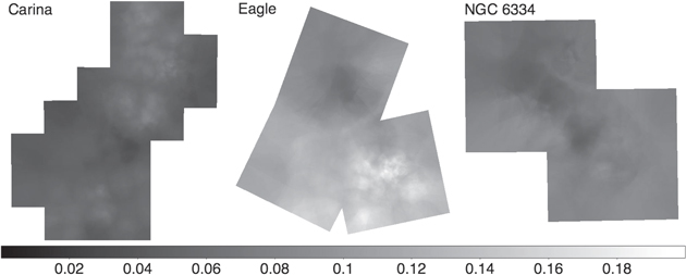