


ABSTRACT
We present the first installment of a massive spectroscopic survey of Galactic O stars, based on new, high signal-to-noise ratio, R ∼ 2500 digital observations from both hemispheres selected from the Galactic O-Star Catalog of Maíz Apellániz et al. and Sota et al. The spectral classification system is rediscussed and a new atlas is presented, which supersedes previous versions. Extensive sequences of exceptional objects are given, including types Ofc, ON/OC, Onfp, Of?p, Oe, and double-lined spectroscopic binaries. The remaining normal spectra bring this first sample to 184 stars, which is close to complete to B = 8 and north of δ = −20° and includes all of the northern objects in Maíz Apellániz et al. that are still classified as O stars. The systematic and random accuracies of these classifications are substantially higher than previously attainable, because of the quality, quantity, and homogeneity of the data and analysis procedures. These results will enhance subsequent investigations in Galactic astronomy and stellar astrophysics. In the future, we will publish the rest of the survey, beginning with a second paper that will include most of the southern stars in Maíz Apellániz et al.
Export citation and abstract BibTeX RIS
1. INTRODUCTION
In Maíz Apellániz et al. (2004), we presented the first version of the Galactic O-Star Catalog (GOSC), a collection of spectral classifications for 378 Galactic O stars accompanied by astrometric, photometric, group membership, and multiplicity information. Most of the stars in that first version had been classified by one of us (N.R.W.) two or three decades earlier using photographic spectrograms. GOSC was subsequently expanded (version 2) by Sota et al. (2008), who added ∼1000 stars that had at least one spectral classification in the literature that identified them as O stars. As a quick look at the online version12 of GOSC v2 reveals, there is an unfortunately large disparity in the literature spectral classifications for the stars there. Some of the discrepancies are due to different spectral resolutions or signal-to-noise ratios (S/Ns), others to variability in the stars (spectroscopic binaries being the major culprit here), and still others to errors or different criteria among classifiers. We believe it is important to correct this situation, not only for the sake of the analysis of individual stars but also because the use of inconsistent or incorrect spectral classifications may lead to errors in the derivation of statistically based parameters such as the massive-star initial mass function or the overall number of ionizing photons in the Galaxy.
Thus was born in 2007 the idea for the Galactic O-Star Spectroscopic Survey (GOSSS), a project whose primary goal is to obtain new spectral classifications of at least all Galactic O stars brighter than B = 13. Since then, we are deriving classifications using new, uniform quality, high-S/N spectrograms homogeneously processed and classified according to well-defined standards. The survey is described in Maíz Apellániz et al. (2010).
How opportune and feasible is such a project? On the one hand, we are in a better position to do it than when similar surveys were attempted in the 1960s and 1970s: there are more telescopes, better detectors, improved data reduction software, and much larger reference databases. Furthermore, many of the targets are relatively bright, making the project accessible to 1–4 m class telescopes. On the other hand, such a project still represents a large and complicated endeavor, with the targets scattered along the Galactic Plane in two hemispheres and requiring hundreds of observation nights. Also, since most fields include none or only a few additional O stars within ∼10' of the primary target, the use of a fiber spectrograph would be a waste of resources and a complication for harmonizing the data from different observatories. Hence, the project is being conducted using long-slit spectrographs.
The earliest results from GOSSS were presented in a letter (Walborn et al. 2010a) that discussed the presence of the C iii λ4650 blend in Of spectra. In this first paper, we present (1) an overview of the project, (2) an atlas of the blue-violet spectral classification standards at R ∼ 2500 from both hemispheres that will be the basis of the rest of the survey, and (3) a spectral library of 184 O stars without Wolf–Rayet (WR) companions and with declinations larger than −20°. The majority of the stars in this paper are from Maíz Apellániz et al. (2004); a few have been added to achieve completeness13 to B = 8.0, because of their presence in the same slit as other O stars, or because of their inclusion in Walborn et al. (2010a). The declination limit is fixed by the accessibility from our northern observatories but it turns out to be a useful value because it splits the numbers in the original catalog into two nearly equal parts. Paper II will be the complement of part (3) of this one for declinations smaller than −20°. Future papers will extend the O-star sample and the wavelength coverage; in both cases we already have abundant data taken.14 We may also publish the spectrograms of the hundreds of non-O and low-mass stars (B,15 WR—including WNh stars16—hot subdwarfs) and the handful of O + WR systems that we are obtaining as byproducts of our search.
2. SURVEY DESCRIPTION
2.1. Blue-violet Spectroscopy with R ∼ 2500
The primary goal of GOSSS is to obtain high-S/N (200–300) blue-violet spectrograms of all O stars with B < 13 at a high degree of uniformity and R ∼ 2500. Given those conditions, our first step was to select the telescopes and instruments with which to carry on the survey. For the northern part of the survey, we settled on the Albireo spectrograph17 at the 1.5 m telescope of the Observatorio de Sierra Nevada (OSN), which can reach stars down to δ = −20°. For the southern part of the survey (δ < −20°), we chose the Boller & Chivens spectrograph18 at the 2.5 m du Pont telescope at Las Campanas Observatory (LCO). The du Pont telescope can reach the desired S/N values for the dimmest stars in the sample within a reasonable total integration time (approximately 1 hr), but in the north the 1.5 m at OSN requires significantly longer exposure times, which compromise the quality of the spectra due to the required instrument stability. Therefore, the dimmer stars (B>11) in the northern part of the survey were observed with the TWIN spectrograph19 at the 3.5 m telescope of Calar Alto Observatory (CAHA, Centro Astronómico Hispano Alemán). Also, since the image quality (seeing+telescope+instrument) is usually better with TWIN at CAHA than with Albireo at OSN, some of the bright northern stars with close companions were observed from CAHA in order to better spatially separate the two spectra.
The characteristics of the three setups are shown in Table 1. We used observations of the same stars with two or three of the telescopes to check the uniformity of the data.20 The spectral resolution of our OSN and LCO observations as measured from the arc spectra turned out to be very similar and stable from night to night. R4500 = 4500 Å/Δλ = 2500 ± 100 with Δλ, the FWHM of the calibration lamp emission lines, being nearly constant over the full wavelength range with a value of 1.8 Å. For our CAHA data, the spectral resolution was somewhat higher (R4500 ∼ 3000, Δλ ∼ 1.5 Å) and with a different dependence on wavelength. In order to provide a uniform spectral library, a smoothing filter was applied to the CAHA data to achieve a constant Δλ = 1.8 Å for the full spectral range.
Table 1. Telescopes, Instruments, and Settings Used
| Telescope | Spectrograph | Grating | Spectral Scale | Spatial Scale | Wav. Range |
|---|---|---|---|---|---|
| (l mm−1) | (Å pixel−1) | ('' pixel−1) | (Å) | ||
| OSN 1.5 m | Albireo | 1800 | 0.66 | 0.85 | 3740–5090 |
| LCO 2.5 m (du Pont) | Boller & Chivens | 1200 | 0.80 | 0.56 | 3900–5510 |
| CAHA 3.5 m | TWIN (blue arm) | 1200 | 0.54 | 0.69 | 3930–5020 |
Download table as: ASCIITypeset image
In this paper, we present mostly OSN and CAHA data, since the majority of the results here correspond to the northern part of the survey. Nevertheless, the atlas includes LCO data because for some spectral types southern standards are better than northern ones.21 Our goal is to maintain our telescope triad for at least the part of the survey for Paper II. If we eventually include new telescopes and/or instruments, we will first check for uniformity with the existing data.
The data in this paper were obtained between 2007 and 2010. In some cases, observations were repeated due to focus and other instrument issues detected after the fact. For SB2 and SB3 spectroscopic binaries, multiple epochs were obtained to observe the different orbit phases. In most cases with known orbits, observations near quadrature were attempted.
In order to reduce the large amount of data in GOSSS, one of us (A.S.) wrote a pipeline in IDL. The pipeline first applies the bias and flat and calculates a mask to eliminate cosmic rays and cosmetic defects. Second, the data are calibrated in wavelength and placed into the star rest frame. Third, the star(s) in each long-slit exposure is/are identified and extracted. Then, the spectra from different exposures (three or four per target) are combined and the final spectrogram is finally rectified. The pipeline can be run in either (1) a fully automated mode that is usually good enough for a quick look at the telescope or (2) an interactive mode that allows for the tweaking of some parameters such as the mask calculation or the spectrum rectification.
A special case is that of close pairs with small magnitude differences (Δm). For those systems, we aligned the slit parallel to the line joining the two stars to include both of them and we used a custom-made IDL fitting routine derived from the MULTISPEC code (Maíz Apellániz 2005) to deconvolve the two spatial profiles and extract the spectra for the two stars. An example is shown in Figure 1. The procedure works very well for large separations but becomes increasingly harder for small values, especially if Δm is large or the seeing is degraded. The closest pair for which we were able to extract separate spectra thanks to excellent seeing conditions was HD 17 520 AB (Δm ≈ 0.7 mag) with a separation of 0 316 (Maíz Apellániz 2010). On the other hand, we were unable to separate σ Ori AB, which currently has a slightly lower separation (0260) but a significantly larger Δm (≈1.6 mag; Maíz Apellániz 2010). As will be shown later, the use of such a deconvolution technique is the reason for the largest changes in the spectral classifications in this paper with respect to previous works.

Figure 1. Top left: false-color representation of a portion of a GOSSS long-slit exposure of HD 190 429 A+B. The spectral direction is nearly parallel to the x-axis. The bottom (brighter) component is A and the top (weaker) component is B. Top right: spatial intensity cuts for two different wavelengths (one in red and one in blue) for the data on the top left panel. The dotted lines show the two-component fit to the data. Bottom: rectified extracted spectrum for each component and for the sum of the two. The continua are all normalized to the value of the A component (ΔBTy = 0.679 mag). Note the appearance of C iii λ4647-50-51 and He i λ4713 absorptions and the change in the He ii λ4686 profile for the A+B spectrum when compared to that of the A component.
Download figure:
Standard image High-resolution imageThe data from each observatory cover slightly different wavelength ranges (Table 1). The spectrograms shown in this paper have been cut to show the same spectral range.
2.2. Complementary Data, Nomenclature, and Cataloguing
Two problems that have complicated the spectral classification of massive stars in the past are (1) the presence of nearby resolved companions that may or may not contribute to the observed primary spectrum depending on the magnitude difference, separation, slit orientation, and seeing; and (2) the misidentification of components in multiple systems. Both issues are known to be the sources of some discrepancies between literature spectral classifications of the same target.
In order to correct those two issues as much as possible, we used two strategies. On the one hand, we analyzed high-resolution imaging to identify and measure the magnitude differences of nearby companions. For the northern part of the survey, this was done with Lucky-Imaging AstraLux observations at the 2.2 m telescope of CAHA and Hubble Space Telescope (HST) imaging (GO programs 10602 and 11981, PI: Maíz Apellániz, and archival data). The first results appeared in Maíz Apellániz (2010) and will be used here. For the southern part of the survey, we will use, among others, HST imaging from programs 10205 (PI: Walborn), 10602, and 10898 (PI: Maíz Apellániz). On the other hand, we searched the literature for results similar to those obtained with AstraLux (e.g., McCaughrean & Stauffer 1994; Duchêne et al. 2001; Mason et al. 1998, 2009; Turner et al. 2008; Bouy et al. 2008) and we plotted information from Simbad using Aladin images to ensure the correct identification of sources. In order to minimize possible future confusions, we provide charts for some specific cases. We followed the component nomenclature of the Washington Double Star Catalog (Mason et al. 2001).
In some cases, the information derived from the sources above allowed us to determine whether two or more visual components are spatially unresolved in our data. We considered that a secondary component is capable of significantly modifying the spectral type if |ΔB| ⩽ 2.0. In such cases we included in the name of the star the two components (e.g., Pismis 24–1 AB or HD 93 129 AaAb); for larger values of |ΔB| the secondary component was not included in the name. Note that when we are able to spatially resolve a nearby component and extract its spectrum independently from the primary, we do include the component name in each case (e.g., HD 218 195 A) even if |ΔB| is larger than 2.0.
As previously mentioned, the GOSSS sample was drawn from version 2.3 of GOSC (Sota et al. 2008). Our plans for the future include using the new spectral classification to produce a new (3.0) version of the catalog. That version will include not only the spectral classifications but the spectroscopic data themselves as well as the new distances (Maíz Apellániz et al. 2008) derived from the new Hipparcos data reduction (van Leeuwen 2007).
2.3. Spectral Classification Methodology
Spectral classification according to the Morgan–Keenan (MK) process is carried out by (1) selecting a two-dimensional grid (in spectral type and luminosity class) of standard stars; (2) comparing the unknown spectrum with that grid, in terms of the line ratios that define the different subtypes; and (3) choosing the standard spectrum that most resembles the unknown spectrum, if appropriate noting any anomalies such as broad lines or discrepancies among different line ratios compared to the standards. The classification categories are discrete, whereas the phenomena are continuous, so interpolations or compromises may be required in some cases, which should be noted.
Many of the stars we selected as standard stars for this paper have been previously used as such, in some cases going back to the original definition of the O subtypes. Nevertheless, in some cases we noted inconsistencies that made us revise the spectral classification, or we found other, superior definitions of the category among our expanded sample, as detailed in the next section. For the comparison between the unknown spectra and the standards we used MGB,22 an IDL code developed by one of us (J.M.A.) that overplots the two and allows the user to easily change from one standard to another. MGB also allows the user to artificially broaden the standard spectra to measure the line broadening (see next section) and also to combine two standard spectra adjusting their velocities and flux fraction in order to analyze spectroscopic binaries (see Figure 2 for two examples). The software was independently used by two of the authors and the results compared. In most cases there was an excellent agreement in the classifications; discrepancies were subsequently analyzed in more detail.

Figure 2. Two examples of spectral classifications of double-lined spectroscopic binaries using MGB. The bottom (black) line shows the spectrum to be classified and the top (red or gray) line the linear combination of the two standards. The flux fraction and velocity of each standard are indicated along with its spectral type.
Download figure:
Standard image High-resolution imageOne important aspect is that spectral classification is subject to the effects of spectral, spatial, and temporal resolution as well as S/N. For example, an SB2 may remain undetected without adequate resolution or temporal coverage, possibly yielding anomalously wide lines due to blends; in other cases some absorption lines may be too weak to be detected, e.g., He ii λ4542 at B0. In other cases, a close visual binary may have historical composite spectra (hence, intermediate spectral classifications and/or peculiarities) that cannot be separated until spatially resolved spectroscopy can be obtained. Such limitations are a major reason for discrepant spectral classifications in the literature. As previously described, we are taking steps to minimize such effects (e.g., obtaining multiple-epoch spectroscopy for known SB2s and to discover new ones), but it is impossible to eliminate them completely. That is one of the reasons why we publish not only the spectral types, but also the original spectrograms, since that enables comparison with past or future results. In that regard, we have searched the literature for spectrograms that may be in conflict with our classifications (because of, e.g., better temporal or spectral resolution) and analyzed those cases. We plan to continually update the GOSC whenever new data justify it in the future.
3. RESULTS
This section constitutes the main body of this paper and is divided in three parts. First, we present the new atlas of standard O stars and the associated spectral classification developments. Second, we briefly present the noteworthy characteristics of some of the members of the peculiar categories (Ofc, ON/OC, Onfp, Of?p, Oe, SB2+SB3) of the full Northern sample (atlas and non-atlas stars) in the paper. Finally, we do the same with the normal O stars in the full Northern sample.
3.1. Atlas and Spectral Classification System Developments
A historical and technical review of the current spectral classification system for the OB stars was given by Walborn (2009). Because of the unprecedented quality and quantity of the present data set, several systemic developments and revisions for the O stars are introduced in the present work, which supersede previous procedures and are described here. Classification standards are listed in Table 2, and an extensive new spectral atlas is presented in Figures 3–11; the first four figures provide spectral-type sequences at fixed luminosity classes, while the latter five are luminosity-class sequences at fixed spectral types (with a few exceptions because of positions unrepresented in the current sample).23 This atlas replaces that of Walborn & Fitzpatrick (1990) for the O spectral types. A list of qualifiers for O spectral types is provided in Table 3.

Download figure:
Standard image High-resolution image
Figure 3. Atlas of rectified digital, linear-intensity spectrograms for luminosity class I, Galactic O stars. In this and subsequent figures, the y-axis is labeled in continuum units and the spectrograms are vertically displaced for display purposes.
Download figure:
Standard image High-resolution image
Figure 4. Same as Figure 3 for luminosity class II.
Download figure:
Standard image High-resolution image
Download figure:
Standard image High-resolution image
Figure 5. Same as Figure 3 for luminosity class III.
Download figure:
Standard image High-resolution image
Download figure:
Standard image High-resolution image
Figure 6. Same as Figure 3 for luminosity class V.
Download figure:
Standard image High-resolution image
Figure 7. Luminosity effects at spectral type O4.
Download figure:
Standard image High-resolution image
Figure 8. Luminosity effects at spectral type O6.5.
Download figure:
Standard image High-resolution image
Figure 9. Luminosity effects at spectral type O8. Note that HD 112 244 is not in our standard list because of its broad lines.
Download figure:
Standard image High-resolution image
Figure 10. Luminosity effects at spectral type O8.5.
Download figure:
Standard image High-resolution image
Figure 11. Luminosity effects at spectral type O9.
Download figure:
Standard image High-resolution imageTable 2. Spectral Classification Standards
| V | IV | III | II | Ib | Iab/I | Ia | |
|---|---|---|---|---|---|---|---|
| O2 | HD 93 129 AaAb | ||||||
| O3 | HD 64 568 | ... | Cyg OB2-7 | ||||
| O3.5 | HD 93 128 | Pismis 24-17 | Pismis 24-1 AB | ||||
| O4 | HD 46 223 | HD 168 076 AB | HD 15 570 | ||||
| HD 96 715 | HD 93 250 | HD 16 691 | |||||
| HD 190 429 A | |||||||
| O4.5 | HD 15 629 | Cyg OB2-8 C | HD 14 947 | ||||
| HDE 303 308 | Cyg OB2-9 | ||||||
| O5 | HD 46 150 | HD 168 112 | CPD -47 2963 | ||||
| HDE 319 699 | HD 93 403 | ||||||
| HD 93 843 | |||||||
| O5.5 | HD 93 204 | ... | Cyg OB2-11 | ||||
| O6 | HD 42 088 | HD 101 190 | ... | HDE 229 196 | ... | ... | HD 169 582 |
| HDE 303 311 | |||||||
| O6.5 | HD 91 572 | HDE 322 417 | HD 190 864 | HD 157 857 | ... | ... | HD 163 758 |
| HD 12 993 | HD 96 946 | ||||||
| HD 152 723 | |||||||
| HD 156 738 | |||||||
| O7 | HD 93 146 | ... | Cyg OB2-4 | HD 94 963 | HD 69 464 | ... | ... |
| HDE 242 926 | HD 151 515 | HD 193 514 | |||||
| HD 91 824 | |||||||
| HD 93 222 | |||||||
| 15 Mon AaAb | |||||||
| O7.5 | HDE 319 703 A | ... | HD 163 800 | HD 34 656 | HD 17 603 | HD 192 639 | ... |
| HD 152 590 | HD 171 589 | HD 156 154 | 9 Sge | ||||
| O8 | HD 191 978 | HD 97 166 | HDE 319 702 | HD 162 978 | BD −11 4586 | HD 225 160 | HD 151 804 |
| HD 97 848 | λ Ori A | ||||||
| O8.5 | HD 46 149 | HD 46 966 | HD 114 737 | HD 75 211 | HD 125 241 | ... | HDE 303 492 |
| HD 57 236 | HD 218 195 A | ||||||
| HD 14 633 | |||||||
| O9 | 10 Lac | CPD -41 7733 | HD 24 431 | τ CMa | 19 Cep | HD 202 124 | α Cam |
| HD 216 898 | HD 93 028 | HD 93 249 | HD 207 198 | HD 148 546 | |||
| HD 193 443 AB | HD 71 304 | HD 152 249 | |||||
| O9.5 | AE Aur | HD 192 001 | HD 96 264 | δ Ori AaAb | HD 76 968 | HD 188 209 | ... |
| HD 46 202 | HD 93 027 | HD 154 368 | |||||
| HD 12 323 | HD 155 889 | HD 123 008 | |||||
| HD 96 622 | |||||||
| O9.7 | υ Ori | HD 207 538 | HD 189 957 | HD 68 450 | V689 Mon | HD 225 146 | HD 195 592 |
| HD 154 643 | HD 152 405 | HD 75 222 | HD 173 010 | ||||
| HD 10 125 | μ Nor | HD 105 056 | |||||
| HD 152 424 | |||||||
| B0 | τ Sco | ... | HD 48 434 | ... | ... | ... | ε Ori |
| HD 122 879 | |||||||
| B0.2 | HD 2083 | ϕ1 Ori | HD 6675 | ... | ... | ... | ... |
| B0.5 | HD 36 960 | ... | 1 Cas | ... | ... | ... | κ Ori |
Notes. Normal, italic, and bold typefaces are used for stars with δ> + 20°, δ < −20°, and the equatorial in-between region, respectively. υ Ori, a previous B0 V standard, is now an O9.7 V. τ Sco, a previous B0.2 V standard, is now a B0 V. HD 189 957, a previous O9.5 III standard is now an O9.7 III.
Download table as: ASCIITypeset image
Table 3. Qualifiers used for Spectral Classification in this Work and in Others
| Qualifier | Description |
|---|---|
| ((f)) | Weak N iii λ4634-40-42 emission, strong He ii λ4686 absorption |
| (f) | Medium N iii λ4634-40-42 emission, neutral or weak He ii λ4686 absorption |
| f | Strong N iii λ4634-40-42 emission, He ii λ4686 emission above continuum |
| ((f*)) | N iv λ4058 emission ⩾ N iii λ4640 emission, strong He ii λ4686 absorption (O2-3.5) |
| (f*) | N iv λ4058 emission ⩾ N iii λ4640 emission, weaker He ii λ4686 absorption (O2-3.5) |
| f* | N iv λ4058 emission ⩾ N iii λ4640 emission, He ii λ4686 emission (O2-3.5) |
| ((fc)) | As ((f)) plus C iii λ4647-50-51 emission equal to N iii λ4634 |
| (fc) | As (f) plus C iii λ4647-50-51 emission equal to N iii λ4634 |
| fc | As f plus C iii λ4647-50-51 emission equal to N iii λ4634 |
| f?p | Variable C iii λ4647-50-51 emission ⩾ N iii λ4634-40-42 at maximum; variable |
| sharp absorption, emission, and/or P Cygni features at H and He i lines | |
| ((f+)) | As ((f)) plus Si iv λ4089-4116 emission (O4-8, obsolete, see Section 3.1.3) |
| (f+) | As (f) plus Si iv λ4089-4116 emission (O4-8, obsolete, see Section 3.1.3) |
| f+ | As f plus Si iv λ4089-4116 emission (O4-8, obsolete, see Section 3.1.3) |
| (e) | Probable Hα emission but no red spectrogram available |
| e | Emission components in H lines |
| pe | As e with emission components in He i and/or continuum veiling |
| [e] | Emission spectrum including Fe forbidden lines |
| e+ | Fe ii and H emission lines (subcategories in Lesh 1968) |
| ((n)) | Broadened lines (not applied here, marginal) |
| (n) | More broadened lines (vsin i ∼ 200 km s−1) |
| n | Even more broadened lines (vsin i ∼ 300 km s−1) |
| nn | Yet even more broadened lines (vsin i ∼ 400 km s−1) |
| [n] | H lines more broadened than He lines |
| nfp | He ii centrally reversed emission, broadened absorption lines (Conti Oef) |
| N | N absorption enhanced, C and O deficient |
| Nstr | Moderate case of above (e.g., N iii λ4640 enhanced but not > C iii λ4650) |
| C | C absorption enhanced, N deficient |
| Nwk | Moderate case of above |
| var | Variation in line spectrum intensities or content |
| p | Peculiar spectrum |
| z | He ii λ4686 in absorption and > than both He i λ4471 and He ii λ4542 |
Download table as: ASCIITypeset image
With regard to line broadening, we have consistently distinguished the three degrees (n), n, and nn in this work. The ((n)) qualifier of Walborn (1971) has not been applied, as it was judged too marginal and close to the slight resolution differences among the different instruments involved. Figure 12 shows the sequence from normal to nn stars for stars around type O9 II. See Table 3 for the approximate velocities that correspond to (n), n, and nn, respectively.24

Figure 12. Broadening sequence (normal, (n), n, nn) for four O stars of similar spectral type.
Download figure:
Standard image High-resolution image3.1.1. Spectral-type Criteria at O8–O9
The primary horizontal classification criterion for the O stars has been the helium ionization ratio He ii λ4542/He i λ4471. It has a value of unity at type O7 and is very sensitive toward either side. However, when the ratio becomes very unequal, its estimation is more difficult; nevertheless, it has been applied throughout the O-type sequence. At the earliest types, there is no comparable absorption-line alternative, but at late-O types the ratios He ii λ4542/He i λ4388 and He ii λ4200/He i λ4144 are very sensitive. In previous work, they have been allowed to increase with luminosity class at a given spectral type, but here we adopt them as the primary spectral-type criteria at types O8.5–B0 and define type O9 by values of unity in both of these ratios. As a result, there may be small systematic differences between the present and previous classifications (although Walborn et al. 2000 had already adopted these procedures), and the spectral types of some fundamental standards have been revised, e.g., α Cam and 19 Cep from O9.5 to O9. It is believed that these new definitions will yield more reproducible and consistent classifications for late-O stars. The definition of type O9.7 remains He ii λ4542 equal to Si iii λ4552, with a range from slightly greater to slightly less than allowed. This spectral type was formerly used only for luminosity classes higher than III, but here it has been newly applied at the lower luminosity classes as well, to improve the overall consistency at late-O types. Thus, three standard stars have been moved: HD 189 957 from O9.5 III to O9.7 III, υ Ori from B0 V to O9.7 V, and τ Sco from B0.2 V to B0 V. It is expected that this redefinition will increase the number of stars classified as O by moving previous B0 V to III objects to the O9.7 V to III categories. The criteria at types O8.5–B0 are summarized in Table 4.
Table 4. Spectral-type Criteria at Types O8.5–B0 (Comparisons Between Absorption-line Pairs)
| Spectral | He ii λ4542/He i λ4388 | Si iii λ4552/He ii λ4542 |
|---|---|---|
| Type | and | |
| He ii λ4200/He i λ4144 | ||
| O8 | > | N/A |
| O8.5 | ⩾ | N/A |
| O9 | = | ≪ |
| O9.5 | ⩽ | < |
| O9.7a | < | ⩽ to ⩾ |
| B0 | ≪ | ≫ |
Note. aNow used at all luminosity classes.
Download table as: ASCIITypeset image
3.1.2. Luminosity-class Criteria
The first luminosity classification for stars earlier than types O8–O9 was introduced by Walborn (1971, 1973b); it is based upon the selective emission (Walborn 2001) effects in He ii λ4686 and N iii λλ4634–4640–4642, i.e., the Of effect. It was in part based on the inference that the negative luminosity effect in the corresponding absorption lines at late-O types is caused by emission filling by the same effect. At late-O types, the increasing intensity of the Si iv lines at λλ4089, 4116 relative to nearby He i lines provides an independent luminosity criterion (Table 5). In some spectra, for whatever reasons (e.g., companions, metallicity, resolution effects on lines of different intrinsic widths, etc.), these independent criteria can be somewhat discrepant; examples can be seen in the present atlas and sample. In the MK process, the general approach is to examine the entire spectrum and adopt an "average" over all available criteria; if the discrepancies are judged to be too great, a "p" (for peculiar) is added to the spectral type. Here, we have preferred to adopt the behavior of He ii λ4686 as the primary luminosity criterion for definiteness, allowing some range in the Si iv at a given class. The values of the He ii λ4686/He i λ4713 ratio at spectral types O8–O8.5 and O9–9.7 are given in Tables 5 and 6, respectively; the corresponding morphology at earlier types is defined in the atlas. Again, it is believed that this procedure will yield more reproducible and consistent luminosity classes; the effects on the calibration remain to be investigated.
Table 5. O8–O8.5 He ii λ4686 Luminosity Criterion
| Lum. | O8 | O8.5 |
|---|---|---|
| Class | ||
| Ia | Strong emission | Weak emission |
| Iab | Weak emission | Neutral |
| Ib | Near neutral | Very weak absorption |
| II | Weak absorption | |
| III | Strong absorption | |
| V | Very strong absorption | |
Download table as: ASCIITypeset image
Table 6. O9–O9.7 Luminosity Criteria (Comparisons Between Absorption-line Pairs)
| Lum. | He ii λ4686/He i λ4713 | Si iv λ4089/He i λ4026 |
|---|---|---|
| Class | ||
| Ia | ∼0 | > |
| Iab | ≪ to < | ⩾ to ⩽ |
| Ib | ⩽ | ⩽ |
| II | = | < |
| III | > | < to ≪ |
| V | ≫ | ≪ |
Download table as: ASCIITypeset image
On this basis, we can now readily distinguish luminosity class IV at spectral types O6–O8 in data of the present quality; these types were previously little used if at all. Here, the He ii λ4686 absorption is intermediate between those of classes V and III.25 Inversely, many previously known and new examples of type O Vz (Walborn 2007), in which He ii λ4686 absorption is stronger than any other He ii or He i lines, hypothesized to be caused by an "inverse Of effect" and possibly related to extreme youth, are readily seen in the atlas and normal sample.
3.1.3. Ofc Stars
As already reported by Walborn et al. (2010a), this study has revealed a new category of O-type spectra, denoted as Ofc, in which emission lines of C iii λλ4647–4650–4652 reach intensities similar to the adjacent ones of N iii λλ4634–4640–4642 that are included in the definition of the Of category. This phenomenon is strongly peaked at spectral-type O5 at all luminosity classes and, as discussed in the earlier paper, likely corresponds to a sharply defined sensitivity of the ionic level populations to the atmospheric parameters. Figure 13 here presents the complete violet through green spectral range in the current sample of eight Northern Ofc spectra, and the atlas illustrates the behavior of these features at adjacent spectral types. It can be seen that in some of the hottest Ofc spectra, Si iv λ4654 and C iv λ4658 become comparable to the C iii (see also Walborn et al. 2002).

Figure 13. Spectrograms for Ofc stars.
Download figure:
Standard image High-resolution imageA related notational point is the elimination of the "+" sign following the "f," previously used to denote emission in Si iv λλ4089, 4116. That notation unfortunately created confusion with superluminosity, as used for late-O and early-B supergiants. It is no longer regarded as essential, as the Si iv emission is now well established as a common feature that responds to temperature and gravity in normal O-type spectra, and many other selective emission features are being identified (Walborn 2001; Werner & Rauch 2001; Corti et al. 2009). The degrees of the f-parameter itself are left unchanged and they are still defined in terms of the qualitative appearance of He ii λ4686 and N iii λλ4634–4640–4642 combined, e.g., absorption or emission in the former (see Table 3 for details).
3.2. Peculiar Categories
In this subsection, we describe the characteristics and membership in the sample of this paper of the different peculiar categories of O stars. The spectral classifications of this and the next subsection are shown in Table 7. Stars within these two subsections and in Table 7 are sorted by their GOS ID (see Maíz Apellániz et al. 2004), whose first numbers correspond to the (rounded) Galactic longitude.
Table 7. Spectral Classifications
| Name | GOSSS ID | R.A. (J2000) | Decl. (J2000) | SC | LC | Qual. | Second. | Altern. Classification | Ref. | Sect. | Flag |
|---|---|---|---|---|---|---|---|---|---|---|---|
| ζ Oph | GOS 006.28 + 23.59_01 | 16:37:09.530 | −10:34:01.75 | O9.5 | IV | nn | ... | ... | ... | 3.3 | ch |
| HD 164 438 | GOS 010.35 + 01.79_01 | 18:01:52.279 | −19:06:22.07 | O9 | III | ... | ... | ... | ... | 3.3 | ... |
| HD 167 659 | GOS 012.20 − 01.27_01 | 18:16:58.562 | −18:58:05.20 | O7 | II–III | (f) | ... | ... | ... | 3.3 | ch |
| HD 167 771 | GOS 012.70 − 01.13_01 | 18:17:28.556 | −18:27:48.43 | O7 | III | (f) | O8 III | ... | ... | 3.2.6 | ch |
| HD 157 857 | GOS 012.97 + 13.31_01 | 17:26:17.332 | −10:59:34.79 | O6.5 | II | (f) | ... | ... | ... | 3.3 | ... |
| HD 167 633 | GOS 014.34 − 00.07_01 | 18:16:49.656 | −16:31:04.30 | O6.5 | V | ((f)) | ... | ... | ... | 3.3 | ch |
| HD 165 319 | GOS 015.12 + 03.33_01 | 18:05:58.838 | −14:11:53.01 | O9.7 | Ib | ... | ... | ... | ... | 3.3 | new |
| HD 175 754 | GOS 016.39 − 09.92_01 | 18:57:35.709 | −19:09:11.25 | O8 | II | (n)(f)p | ... | ... | ... | 3.2.3 | ch |
| HD 168 075 | GOS 016.94 + 00.84_01 | 18:18:36.043 | −13:47:36.46 | O7 | V | (n)((f))z | ... | O6.5 V((f)) + B0 1V | S09 | 3.2.6 | ch |
| HD 168 076 AB | GOS 016.94 + 00.84_02 | 18:18:36.421 | −13:48:02.38 | O4 | III | (f) | ... | O3.5 V((f+)) + O7.5 V | S09 | 3.3 | ch |
| BD −13 4927 | GOS 016.98 + 00.85_01 | 18:18:40.091 | −13:45:18.58 | O7 | II | (f) | ... | ... | ... | 3.3 | ch |
| MY Ser | GOS 018.25 + 01.68_01 | 18:18:05.895 | −12:14:33.30 | O8 | Ia | f(n) | O4/5 | O8 I + O5-8 V + O5-8 V | L87 | 3.2.3 | ch |
| BD −12 4979 | GOS 018.25 + 01.69_01 | 18:18:03.112 | −12:14:34.28 | O9.5 | III–IV | ... | ... | ... | ... | 3.3 | new |
| HD 168 112 | GOS 018.44 + 01.62_01 | 18:18:40.868 | −12:06:23.38 | O5 | III | (f) | ... | ... | ... | 3.3 | ... |
| HD 171 589 | GOS 018.65 − 03.09_01 | 18:36:12.640 | −14:06:55.82 | O7.5 | II | (f) | ... | ... | ... | 3.3 | ch |
| HD 166 734 | GOS 018.92 + 03.63_01 | 18:12:24.656 | −10:43:53.03 | O7.5 | Iab | f | ... | O7 Ib(f) + O8-9 I | W73 | 3.2.6 | ch |
| BD −11 4586 | GOS 019.08 + 02.14_01 | 18:18:03.344 | −11:17:38.83 | O8 | Ib | (f) | ... | ... | ... | 3.3 | ... |
| HD 169 582 | GOS 021.33 + 01.20_01 | 18:25:43.147 | −09:45:11.02 | O6 | Ia | f | ... | ... | ... | 3.3 | ch |
| HD 173 010 | GOS 023.73 − 02.49_01 | 18:43:29.710 | −09:19:12.60 | O9.7 | Ia | ... | ... | ... | ... | 3.3 | ... |
| HD 173 783 | GOS 024.18 − 03.34_01 | 18:47:24.183 | −09:18:29.50 | O9 | Iab | ... | ... | ... | ... | 3.3 | ch |
| V442 Sct | GOS 024.53 − 00.85_01 | 18:39:03.776 | −07:51:35.44 | O6.5 | I | (n)fp | ... | ... | ... | 3.2.3 | ch |
| 9 Sge | GOS 056.48 − 04.33_01 | 19:52:21.765 | +18:40:18.75 | O7.5 | Iab | f | ... | ... | ... | 3.3 | ... |
| HDE 344 783 | GOS 059.37 − 00.15_01 | 19:43:06.790 | +23:16:12.40 | O9.7 | III | ... | ... | ... | ... | 3.3 | new |
| HDE 344 782 | GOS 059.40 − 00.14_01 | 19:43:08.900 | +23:18:08.00 | O9.5 | V | ... | ... | ... | ... | 3.3 | new |
| HDE 344 784 A | GOS 059.40 − 00.15_01 | 19:43:10.970 | +23:17:45.38 | O6.5 | V | ((f)) | ... | ... | ... | 3.3 | ch |
| HD 186 980 | GOS 067.39 + 03.66_01 | 19:46:15.902 | +32:06:58.16 | O7.5 | III | ((f)) | ... | ... | ... | 3.3 | ... |
| Cyg X-1 | GOS 071.34 + 03.07_01 | 19:58:21.678 | +35:12:05.81 | O9.7 | Iab | p var | ... | ... | ... | 3.3 | ch |
| HD 190 864 | GOS 072.47 + 02.02_01 | 20:05:39.800 | +35:36:27.98 | O6.5 | III | (f) | ... | ... | ... | 3.3 | ... |
| HD 190 429 B | GOS 072.58 + 02.61_01 | 20:03:29.410 | +36:01:28.58 | O9.5 | II–III | ... | ... | ... | ... | 3.3 | new |
| HD 190 429 A | GOS 072.59 + 02.61_01 | 20:03:29.393 | +36:01:30.53 | O4 | I | f | ... | ... | ... | 3.3 | ch |
| HD 191 201 A | GOS 072.75 + 01.78_01 | 20:07:23.684 | +35:43:05.91 | O9.5 | III | ... | B0 IV | ... | ... | 3.2.6 | ch |
| HD 191 201 B | GOS 072.75 + 01.78_02 | 20:07:23.766 | +35:43:06.01 | O9.7 | III | ... | ... | ... | ... | 3.3 | new |
| HD 191 612 | GOS 072.99 + 01.43_01 | 20:09:28.608 | +35:44:01.31 | O8 | ... | f?p var | ... | ... | ... | 3.2.4 | ch |
| HD 192 639 | GOS 074.90 + 01.48_01 | 20:14:30.429 | +37:21:13.83 | O7.5 | Iab | f | ... | ... | ... | 3.3 | ch |
| HDE 228 766 | GOS 075.19 + 00.96_01 | 20:17:29.703 | +37:18:31.13 | O4 | I | f | O8: II: | ... | ... | 3.2.6 | ch |
| HD 193 443 AB | GOS 076.15 + 01.28_01 | 20:18:51.707 | +38:16:46.50 | O9 | III | ... | ... | ... | ... | 3.3 | ... |
| BD +36 4063 | GOS 076.17 − 00.34_01 | 20:25:40.608 | +37:22:27.08 | ON9.7 | Ib | ... | ... | ... | ... | 3.2.2 | ch |
| HDE 228 841 | GOS 076.60 + 01.68_01 | 20:18:29.692 | +38:52:39.76 | O6.5 | V | n((f)) | ... | ... | ... | 3.3 | ... |
| HD 193 514 | GOS 077.00 + 01.80_01 | 20:19:08.498 | +39:16:24.23 | O7 | Ib | (f) | ... | ... | ... | 3.3 | ... |
| V2011 Cyg | GOS 077.12 + 03.40_01 | 20:12:33.121 | +40:16:05.45 | O4.5 | V | n(f) | ... | ... | ... | 3.3 | ch |
| Y Cyg | GOS 077.25 − 06.23_01 | 20:52:03.577 | +34:39:27.51 | O9.5 | IV | ... | O9.5 IV | ... | ... | 3.2.6 | ch |
| HDE 229 232 | GOS 077.40 + 00.93_01 | 20:23:59.183 | +39:06:15.27 | O4 | V | n((f)) | ... | ... | ... | 3.3 | ... |
| HD 189 957 | GOS 077.43 + 06.17_01 | 20:01:00.005 | +42:00:30.83 | O9.7 | III | ... | ... | ... | ... | 3.3 | ch |
| HD 191 978 | GOS 077.87 + 04.25_01 | 20:10:58.281 | +41:21:09.91 | O8 | V | z | ... | ... | ... | 3.3 | ch |
| HD 193 322 AaAb | GOS 078.10 + 02.78_01 | 20:18:06.990 | +40:43:55.46 | O9 | IV | (n) | ... | ... | ... | 3.3 | ch |
| HD 201 345 | GOS 078.44 − 09.54_01 | 21:07:55.416 | +33:23:49.25 | ON9.5 | IV | ... | ... | ... | ... | 3.2.2 | ch |
| HD 192 001 | GOS 078.53 + 04.66_01 | 20:11:01.706 | +42:07:36.39 | O9.5 | IV | ... | ... | ... | ... | 3.3 | ... |
| HD 191 423 | GOS 078.64 + 05.37_01 | 20:08:07.113 | +42:36:21.98 | ON9 | II–III | nn | ... | ... | ... | 3.2.2 | ch |
| HDE 229 196 | GOS 078.76 + 02.07_01 | 20:23:10.787 | +40:52:29.85 | O6 | II | (f) | ... | ... | ... | 3.3 | ch |
| Cyg OB2-5 A | GOS 080.12 + 00.91_01 | 20:32:22.422 | +41:18:18.91 | O7 | Ia | fpe | ... | ... | ... | 3.2.6 | ch |
| V2185 Cyg | GOS 080.14 + 00.74_01 | 20:33:09.600 | +41:13:00.60 | O9.5 | III | n | ... | ... | ... | 3.3 | new |
| Cyg OB2-22 A | GOS 080.14 + 00.75_01 | 20:33:08.767 | +41:13:18.74 | O3 | I | f* | ... | ... | ... | 3.3 | ... |
| Cyg OB2-22 B | GOS 080.14 + 00.75_02 | 20:33:08.842 | +41:13:17.48 | O6 | V | ((f)) | ... | ... | ... | 3.3 | ... |
| Cyg OB2-9 | GOS 080.17 + 00.76_01 | 20:33:10.734 | +41:15:08.25 | O4.5 | I | fc | ... | ... | ... | 3.2.1 | ch |
| NSV 13 148 | GOS 080.21 + 00.76_01 | 20:33:17.480 | +41:17:09.30 | O8 | V | (n) | ... | ... | ... | 3.3 | new |
| Cyg OB2-8 A | GOS 080.22 + 00.79_01 | 20:33:15.078 | +41:18:50.51 | O5 | III | (fc) | ... | O6 + O5.5; see note | D04 | 3.2.1 | ch |
| Cyg OB2-8 B | GOS 080.22 + 00.79_02 | 20:33:14.756 | +41:18:41.79 | O6 | II | (f) | ... | ... | ... | 3.3 | new |
| Cyg OB2-4 | GOS 080.22 + 01.02_01 | 20:32:13.823 | +41:27:11.99 | O7 | III | ((f)) | ... | ... | ... | 3.3 | ... |
| Cyg OB2-8 C | GOS 080.23 + 00.78_01 | 20:33:17.977 | +41:18:31.19 | O4.5 | III | (fc) | ... | ... | ... | 3.2.1 | ch |
| Cyg OB2-8 D | GOS 080.23 + 00.79_01 | 20:33:16.328 | +41:19:02.01 | O9 | V | (n) | ... | ... | ... | 3.3 | new |
| Cyg OB2-7 | GOS 080.24 + 00.80_01 | 20:33:14.112 | +41:20:21.88 | O3 | I | f* | ... | ... | ... | 3.3 | ... |
| Cyg OB2-11 | GOS 080.57 + 00.83_01 | 20:34:08.514 | +41:36:59.42 | O5.5 | I | fc | ... | ... | ... | 3.2.1 | ch |
| HD 188 209 | GOS 080.99 + 10.09_01 | 19:51:59.068 | +47:01:38.44 | O9.5 | Iab | ... | ... | ... | ... | 3.3 | ... |
| HD 191 781 | GOS 081.18 + 06.61_01 | 20:09:50.581 | +45:24:10.44 | ON9.7 | Iab | ... | ... | ... | ... | 3.2.2 | ... |
| HD 195 592 | GOS 082.36 + 02.96_01 | 20:30:34.970 | +44:18:54.87 | O9.7 | Ia | ... | ... | O9.7 I + B | D10 | 3.2.6 | ... |
| HD 199 579 | GOS 085.70 − 00.30_01 | 20:56:34.779 | +44:55:29.01 | O6.5 | V | ((f))z | ... | O6 V((f)) + B1-2 V | W01 | 3.2.6 | ch |
| HD 202 124 | GOS 087.29 − 02.66_01 | 21:12:28.389 | +44:31:54.14 | O9 | Iab | ... | ... | ... | ... | 3.3 | ch |
| 68 Cyg | GOS 087.61 − 03.84_01 | 21:18:27.187 | +43:56:45.40 | O7.5 | III | n((f)) | ... | ... | ... | 3.3 | ch |
| 10 Lac | GOS 096.65 − 16.98_01 | 22:39:15.679 | +39:03:01.01 | O9 | V | ... | ... | ... | ... | 3.3 | ... |
| HD 206 183 | GOS 098.89 + 03.40_01 | 21:38:26.284 | +56:58:25.45 | O9.5 | IV–V | ... | ... | ... | ... | 3.3 | new |
| HD 204 827 AaAb | GOS 099.17 + 05.55_01 | 21:28:57.763 | +58:44:23.20 | O9.7 | III | ... | ... | ... | ... | 3.3 | new |
| HD 206 267 AaAb | GOS 099.29 + 03.74_01 | 21:38:57.618 | +57:29:20.55 | O6.5 | V | ((f)) | O9/B0 V | ... | ... | 3.2.6 | ch |
| HD 210 809 | GOS 099.85 − 03.13_01 | 22:11:38.601 | +52:25:47.95 | O9 | Iab | ... | ... | ... | ... | 3.3 | ... |
| HD 207 538 | GOS 101.60 + 04.67_01 | 21:47:39.790 | +59:42:01.35 | O9.7 | IV | ... | ... | ... | ... | 3.3 | new |
| LZ Cep | GOS 102.01 + 02.18_01 | 22:02:04.576 | +58:00:01.33 | O9 | IV | (n) var | B1: V: | ... | ... | 3.2.6 | ch |
| HD 207 198 | GOS 103.14 + 06.99_01 | 21:44:53.278 | +62:27:38.05 | O9 | II | ... | ... | ... | ... | 3.3 | ... |
| λ Cep | GOS 103.83 + 02.61_01 | 22:11:30.584 | +59:24:52.25 | O6.5 | I | (n)fp | ... | ... | ... | 3.2.3 | ch |
| 19 Cep | GOS 104.87 + 05.39_01 | 22:05:08.791 | +62:16:47.35 | O9 | Ib | ... | ... | ... | ... | 3.3 | ch |
| DH Cep | GOS 107.07 − 00.90_01 | 22:46:54.111 | +58:05:03.55 | O5 | V | ((f)) | O6 V ((f)) | ... | ... | 3.2.6 | ch |
| HD 218 915 | GOS 108.06 − 06.89_01 | 23:11:06.948 | +53:03:29.64 | O9.5 | Iab | ... | ... | ... | ... | 3.3 | ... |
| HD 218 195 A | GOS 109.32 − 01.79_01 | 23:05:12.928 | +58:14:29.34 | O8.5 | III | ... | ... | ... | ... | 3.3 | ch |
| HD 216 532 | GOS 109.65 + 02.68_01 | 22:52:30.555 | +62:26:25.92 | O8.5 | V | (n) | ... | ... | ... | 3.3 | ch |
| HD 216 898 | GOS 109.93 + 02.39_01 | 22:55:42.460 | +62:18:22.83 | O9 | V | ... | ... | ... | ... | 3.3 | ch |
| HD 217 086 | GOS 110.22 + 02.72_01 | 22:56:47.194 | +62:43:37.60 | O7 | V | nn((f)) | ... | ... | ... | 3.3 | ch |
| BD +60 2522 | GOS 112.23 + 00.22_01 | 23:20:44.519 | +61:11:40.53 | O6.5 | ... | (n)fp | ... | ... | ... | 3.2.3 | ch |
| HD 225 146 | GOS 117.23 − 01.24_01 | 00:03:57.504 | +61:06:13.07 | O9.7 | Iab | ... | ... | ... | ... | 3.3 | ch |
| HD 225 160 | GOS 117.44 − 00.14_01 | 00:04:03.796 | +62:13:18.99 | O8 | Iab | f | ... | ... | ... | 3.3 | ch |
| AO Cas | GOS 117.59 − 11.09_01 | 00:17:43.059 | +51:25:59.12 | O9.5 | II | (n) | O8 V | ... | ... | 3.2.3 | ch |
| HD 108 | GOS 117.93 + 01.25_01 | 00:06:03.386 | +63:40:46.75 | O8 | ... | fp var | ... | ... | ... | 3.2.4 | ch |
| HD 5005 A | GOS 123.12 − 06.24_01 | 00:52:49.206 | +56:37:39.49 | O4 | V | ((fc)) | ... | ... | ... | 3.2.1 | ch |
| HD 5005 C | GOS 123.12 − 06.24_02 | 00:52:49.550 | +56:37:36.83 | O8.5 | V | (n) | ... | ... | ... | 3.3 | ch |
| HD 5005 B | GOS 123.12 − 06.24_03 | 00:52:49.390 | +56:37:39.71 | O9.7 | II–III | ... | ... | ... | ... | 3.3 | new |
| HD 5005 D | GOS 123.12 − 06.25_01 | 00:52:48.954 | +56:37:30.83 | O9.5 | V | ... | ... | ... | ... | 3.3 | new |
| BD +60 261 | GOS 127.87 − 01.35_01 | 01:32:32.720 | +61:07:45.84 | O7.5 | III | (n)((f)) | ... | ... | ... | 3.3 | ... |
| HD 10 125 | GOS 128.29 + 01.82_01 | 01:40:52.762 | +64:10:23.13 | O9.7 | II | ... | ... | ... | ... | 3.3 | ... |
| HD 13 022 | GOS 132.91 − 02.57_01 | 02:09:30.067 | +58:47:01.58 | O9.7 | II–III | ... | ... | ... | ... | 3.3 | ch |
| HD 12 323 | GOS 132.91 − 05.87_01 | 02:02:30.126 | +55:37:26.38 | ON9.5 | V | ... | ... | ... | ... | 3.2.2 | ch |
| HD 12 993 | GOS 133.11 − 03.40_01 | 02:09:02.473 | +57:55:55.93 | O6.5 | V | ((f))z | ... | ... | ... | 3.3 | ch |
| HD 13 268 | GOS 133.96 − 04.99_01 | 02:11:29.700 | +56:09:31.70 | ON8.5 | III | n | ... | ... | ... | 3.2.2 | new |
| HD 14 442 | GOS 134.21 − 01.32_01 | 02:22:10.701 | +59:32:58.92 | O5 | ... | n(f)p | ... | ... | ... | 3.2.3 | ... |
| BD +62 424 | GOS 134.53 + 02.46_01 | 02:36:18.221 | +62:56:53.35 | O6.5 | V | (n)((f)) | ... | ... | ... | 3.3 | ch |
| V354 Per | GOS 134.58 − 04.96_01 | 02:15:45.938 | +55:59:46.73 | O9.7 | II | (n) | ... | ... | ... | 3.3 | ch |
| BD +60 497 | GOS 134.58 + 01.04_01 | 02:31:57.087 | +61:36:43.95 | O6.5 | V | ((f)) | O8/B0 V | ... | ... | 3.2.6 | ch |
| BD +60 498 | GOS 134.63 + 00.99_01 | 02:32:10.855 | +61:33:07.95 | O9.7 | II–III | ... | ... | ... | ... | 3.3 | new |
| BD +60 499 | GOS 134.64 + 01.00_01 | 02:32:16.752 | +61:33:15.07 | O9.5 | V | ... | ... | ... | ... | 3.3 | ... |
| BD +60 501 | GOS 134.71 + 00.94_01 | 02:32:36.272 | +61:28:25.60 | O7 | V | (n)((f))z | ... | ... | ... | 3.3 | ch |
| HD 15 558 A | GOS 134.72 + 00.92_01 | 02:32:42.536 | +61:27:21.56 | O4.5 | III | (fc) | ... | O5.5 III(f) + O7 V | D06 | 3.2.1 | ch |
| HD 15 570 | GOS 134.77 + 00.86_01 | 02:32:49.422 | +61:22:42.07 | O4 | I | f | ... | ... | ... | 3.3 | ch |
| HD 15 629 | GOS 134.77 + 01.01_01 | 02:33:20.586 | +61:31:18.18 | O4.5 | V | ((fc)) | ... | ... | ... | 3.2.1 | ch |
| BD +60 513 | GOS 134.90 + 00.92_01 | 02:34:02.530 | +61:23:10.87 | O7 | V | n | ... | ... | ... | 3.3 | ... |
| HD 14 947 | GOS 134.99 − 01.74_01 | 02:26:46.992 | +58:52:33.11 | O4.5 | I | f | ... | ... | ... | 3.3 | ch |
| HD 14 434 | GOS 135.08 − 03.82_01 | 02:21:52.413 | +56:54:18.03 | O5.5 | V | nn((f))p | ... | ... | ... | 3.2.3 | ch |
| HD 16 429 A | GOS 135.68 + 01.15_01 | 02:40:44.951 | +61:16:56.04 | O9 | II–III | (n) | ... | O9.5 II + O8 III-IV + B0 V? | M03 | 3.2.6 | ch |
| HD 15 642 | GOS 137.09 − 04.73_01 | 02:32:56.383 | +55:19:39.07 | O9.5 | II–III | n | ... | ... | ... | 3.3 | ch |
| HD 18 409 | GOS 137.12 + 03.46_01 | 03:00:29.719 | +62:43:19.05 | O9.7 | Ib | ... | ... | ... | ... | 3.3 | ... |
| HD 17 505 A | GOS 137.19 + 00.90_01 | 02:51:07.971 | +60:25:03.88 | O6.5 | III | n((f)) | ... | O6.5 III((f)) + O7.5 V((f)) + O7.5 V((f)) | H06 | 3.2.6 | ch |
| HD 17 505 B | GOS 137.19 + 00.90_02 | 02:51:08.263 | +60:25:03.78 | O8 | V | ... | ... | ... | ... | 3.3 | new |
| HD 17 520 A | GOS 137.22 + 00.88_01 | 02:51:14.434 | +60:23:09.97 | O8 | V | ... | ... | ... | ... | 3.3 | ch |
| HD 17 520 B | GOS 137.22 + 00.88_02 | 02:51:14.397 | +60:23:10.12 | O9: | V | e | ... | ... | ... | 3.2.5 | new |
| BD +60 586 A | GOS 137.42 + 01.28_01 | 02:54:10.672 | +60:39:03.59 | O7 | V | z | ... | ... | ... | 3.3 | ch |
| HD 15 137 | GOS 137.46 − 07.58_01 | 02:27:59.811 | +52:32:57.60 | O9.5 | II–III | n | ... | ... | ... | 3.3 | ch |
| HD 16 691 | GOS 137.73 − 02.73_01 | 02:42:52.028 | +56:54:16.45 | O4 | I | f | ... | ... | ... | 3.3 | ch |
| HD 16 832 | GOS 138.00 − 02.88_01 | 02:44:12.717 | +56:39:27.23 | O9.5 | II–III | ... | ... | ... | ... | 3.3 | ch |
| HD 18 326 | GOS 138.03 + 01.50_01 | 02:59:23.171 | +60:33:59.50 | O6.5 | V | (n)((f)) | O9/B0 V: | ... | ... | 3.2.6 | ch |
| HD 17 603 | GOS 138.77 − 02.08_01 | 02:51:47.798 | +57:02:54.46 | O7.5 | Ib | (f) | ... | ... | ... | 3.3 | ... |
| CC Cas | GOS 140.12 + 01.54_01 | 03:14:05.333 | +59:33:48.50 | O8.5 | III | (n)((f)) | ... | O8.5 III + B0 V | H94 | 3.2.6 | ch |
| HD 14 633 | GOS 140.78 − 18.20_01 | 02:22:54.293 | +41:28:47.72 | ON8.5 | V | ... | ... | ... | ... | 3.2.2 | ch |
| α Cam | GOS 144.07 + 14.04_01 | 04:54:03.011 | +66:20:33.58 | O9 | Ia | ... | ... | ... | ... | 3.3 | ch |
| HDE 237 211 | GOS 147.14 + 02.97_01 | 04:03:15.652 | +56:32:24.85 | O9 | Ib | ... | ... | ... | ... | 3.3 | ch |
| HD 24 431 | GOS 148.84 − 00.71_01 | 03:55:38.420 | +52:38:28.75 | O9 | III | ... | ... | ... | ... | 3.3 | ... |
| NGC 1624-2 | GOS 155.36 + 02.61_01 | 04:40:37.266 | +50:27:40.96 | O7 | ... | f?p | ... | ... | ... | 3.2.4 | new |
| ξ Per | GOS 160.37 − 13.11_01 | 03:58:57.900 | +35:47:27.72 | O7.5 | III | (n)((f)) | ... | ... | ... | 3.3 | ... |
| X Per | GOS 163.08 − 17.14_01 | 03:55:23.078 | +31:02:45.04 | O9.5: | ... | npe | ... | ... | ... | 3.2.5 | ch |
| HD 41 161 | GOS 164.97 + 12.89_01 | 06:05:52.456 | +48:14:57.41 | O8 | V | n | ... | ... | ... | 3.3 | ... |
| BD +39 1328 | GOS 169.11 + 03.60_01 | 05:32:13.845 | +40:03:57.88 | O8.5 | Iab | (n)(f) | ... | ... | ... | 3.3 | ch |
| HD 34 656 | GOS 170.04 + 00.27_01 | 05:20:43.080 | +37:26:19.23 | O7.5 | II | (f) | ... | ... | ... | 3.3 | ch |
| AE Aur | GOS 172.08 − 02.26_01 | 05:16:18.149 | +34:18:44.34 | O9.5 | V | ... | ... | ... | ... | 3.3 | ... |
| HD 36 483 | GOS 172.29 + 01.88_01 | 05:33:41.154 | +36:27:34.97 | O9.5 | IV | (n) | ... | ... | ... | 3.3 | ch |
| LY Aur A | GOS 172.76 + 00.61_01 | 05:29:42.647 | +35:22:30.07 | O9.5 | II | ... | O9 III | ... | ... | 3.2.6 | ch |
| HD 35 619 | GOS 173.04 − 00.09_01 | 05:27:36.146 | +34:45:18.97 | O7.5 | V | ((f)) | ... | ... | ... | 3.3 | ch |
| HD 37 737 | GOS 173.46 + 03.24_01 | 05:42:31.160 | +36:12:00.50 | O9.5 | II–III | (n) | ... | ... | ... | 3.3 | ch |
| HDE 242 908 | GOS 173.47 − 01.66_01 | 05:22:29.302 | +33:30:50.43 | O4.5 | V | (n)((fc)) | ... | ... | ... | 3.2.1 | ch |
| BD +33 1025 | GOS 173.56 − 01.66_01 | 05:22:44.001 | +33:26:26.65 | O7 | V | (n)z | ... | ... | ... | 3.3 | new |
| HDE 242 935 A | GOS 173.58 − 01.67_01 | 05:22:46.539 | +33:25:11.28 | O6.5 | V | ((f))z | ... | ... | ... | 3.3 | ch |
| HDE 242 926 | GOS 173.65 − 01.74_01 | 05:22:40.099 | +33:19:09.37 | O7 | V | z | ... | ... | ... | 3.3 | ch |
| HD 37 366 A | GOS 177.63 − 00.11_01 | 05:39:24.799 | +30:53:26.75 | O9.5 | IV | ... | ... | O9.5 V + B0 1V | B07 | 3.2.6 | ch |
| HD 93 521 | GOS 183.14 + 62.15_01 | 10:48:23.511 | +37:34:13.09 | O9.5 | III | nn | ... | ... | ... | 3.3 | ch |
| HD 36 879 | GOS 185.22 − 05.89_01 | 05:35:40.527 | +21:24:11.72 | O7 | V | (n)((f)) | ... | ... | ... | 3.3 | ch |
| HD 42 088 | GOS 190.04 + 00.48_01 | 06:09:39.574 | +20:29:15.46 | O6 | V | ((f))z | ... | ... | ... | 3.3 | ch |
| HD 44 811 | GOS 192.40 + 03.21_01 | 06:24:38.354 | +19:42:15.83 | O7 | V | (n)z | ... | ... | ... | 3.3 | ch |
| V1382 Ori | GOS 194.07 − 05.88_01 | 05:54:44.731 | +13:51:17.06 | O6 | V: | [n]pe var | ... | ... | ... | 3.2.5 | ... |
| HD 41 997 | GOS 194.15 − 01.98_01 | 06:08:55.821 | +15:42:18.18 | O7.5 | V | n((f)) | ... | ... | ... | 3.3 | ch |
| λ Ori A | GOS 195.05 − 12.00_01 | 05:35:08.277 | +09:56:02.96 | O8 | III | ((f)) | ... | ... | ... | 3.3 | ... |
| HD 45 314 | GOS 196.96 + 01.52_01 | 06:27:15.777 | +14:53:21.22 | O9: | ... | npe | ... | ... | ... | 3.2.5 | ch |
| HD 60 848 | GOS 202.51 + 17.52_01 | 07:37:05.731 | +16:54:15.29 | O8: | V: | pe | ... | ... | ... | 3.2.5 | ch |
| 15 Mon AaAb | GOS 202.94 + 02.20_01 | 06:40:58.656 | +09:53:44.71 | O7 | V | ((f)) var | ... | ... | ... | 3.3 | ch |
| δ Ori AaAb | GOS 203.86 − 17.74_01 | 05:32:00.401 | −00:17:56.73 | O9.5 | II | Nwk | ... | O9.5 II + B0.5 III | H02 | 3.2.2 | ch |
| HD 46 966 | GOS 205.81 − 00.55_01 | 06:36:25.887 | +06:04:59.47 | O8.5 | IV | ... | ... | ... | ... | 3.3 | ch |
| HD 47 129 | GOS 205.87 − 00.31_01 | 06:37:24.042 | +06:08:07.38 | O8 | ... | fp var | ... | O8 III/I + O7.5 III | L08 | 3.2.3 | ch |
| HD 46 106 | GOS 206.20 − 02.09_01 | 06:31:38.395 | +05:01:36.38 | O9.7 | II–III | ... | ... | ... | ... | 3.3 | new |
| HD 48 099 | GOS 206.21 + 00.80_01 | 06:41:59.231 | +06:20:43.54 | O6.5 | V | (n)((f)) | ... | O5.5 V ((f)) + O9 V | M10 | 3.2.6 | ch |
| HD 46 149 | GOS 206.22 − 02.04_01 | 06:31:52.533 | +05:01:59.19 | O8.5 | V | ... | ... | O8 V + B0 1V | M09 | 3.2.6 | ... |
| HD 46 202 | GOS 206.31 − 02.00_01 | 06:32:10.471 | +04:57:59.79 | O9.5 | V | ... | ... | ... | ... | 3.3 | ch |
| HD 46 150 | GOS 206.31 − 02.07_01 | 06:31:55.519 | +04:56:34.27 | O5 | V | ((f))z | ... | ... | ... | 3.3 | ch |
| HD 46 056 A | GOS 206.34 − 02.25_01 | 06:31:20.862 | +04:50:03.85 | O8 | V | n | ... | ... | ... | 3.3 | ch |
| HD 46 223 | GOS 206.44 − 02.07_01 | 06:32:09.306 | +04:49:24.73 | O4 | V | ((f)) | ... | ... | ... | 3.3 | ch |
| ζ Ori A | GOS 206.45 − 16.59_01 | 05:40:45.527 | −01:56:33.26 | O9.5 | Ib | Nwk var | ... | ... | ... | 3.2.2 | ch |
| ζ Ori B | GOS 206.45 − 16.59_02 | 05:40:45.571 | −01:56:35.59 | O9.5 | II–III | (n) | ... | ... | ... | 3.3 | new |
| σ Ori AB | GOS 206.82 − 17.34_01 | 05:38:44.768 | −02:36:00.25 | O9.7 | III | ... | ... | ... | ... | 3.3 | ch |
| HD 46 485 | GOS 206.90 − 01.84_01 | 06:33:50.957 | +04:31:31.61 | O7 | V | n | ... | ... | ... | 3.3 | ch |
| HD 46 573 | GOS 208.73 − 02.63_01 | 06:34:23.568 | +02:32:02.94 | O7 | V | ((f))z | ... | ... | ... | 3.3 | ch |
| θ1 Ori CaCb | GOS 209.01 − 19.38_01 | 05:35:16.463 | −05:23:23.18 | O7 | V | p | ... | ... | ... | 3.3 | ... |
| θ2 Ori A | GOS 209.05 − 19.37_01 | 05:35:22.900 | −05:24:57.79 | O9.5 | IV | p | ... | ... | ... | 3.3 | ch |
| ι Ori | GOS 209.52 − 19.58_01 | 05:35:25.981 | −05:54:35.64 | O9 | III | var | ... | O9 III + B1 III | S87 | 3.2.6 | ch |
| V689 Mon | GOS 210.03 − 02.11_01 | 06:38:38.187 | +01:36:48.66 | O9.7 | Ib | ... | ... | ... | ... | 3.3 | ... |
| HD 48 279 A | GOS 210.41 − 01.17_01 | 06:42:40.548 | +01:42:58.23 | O8.5 | V | Nstr var? | ... | ... | ... | 3.2.2 | ch |
| υ Ori | GOS 210.44 − 20.99_01 | 05:31:55.860 | −07:18:05.53 | O9.7 | V | ... | ... | ... | ... | 3.3 | new |
| HD 52 533 A | GOS 216.85 + 00.80_01 | 07:01:27.048 | −03:07:03.28 | O8.5 | IV | n | ... | ... | ... | 3.3 | ch |
| HD 52 266 | GOS 219.13 − 00.68_01 | 07:00:21.077 | −05:49:35.95 | O9.5 | III | n | ... | ... | ... | 3.3 | ch |
| HD 54 662 | GOS 224.17 − 00.78_01 | 07:09:20.249 | −10:20:47.64 | O7 | V | ((f))z var? | ... | O6.5 V + O7–9.5 V | B07 | 3.2.6 | ch |
| HD 57 682 | GOS 224.41 + 02.63_01 | 07:22:02.053 | −08:58:45.77 | O9.5 | IV | ... | ... | ... | ... | 3.3 | ch |
| HD 55 879 | GOS 224.73 + 00.35_01 | 07:14:28.253 | −10:18:58.50 | O9.7 | III | ... | ... | ... | ... | 3.3 | ch |
| HD 54 879 | GOS 225.55 − 01.28_01 | 07:10:08.149 | −11:48:09.86 | O9.7 | V | ... | ... | ... | ... | 3.3 | ch |
| HD 53 975 | GOS 225.68 − 02.32_01 | 07:06:35.964 | −12:23:38.23 | O7.5 | V | z | ... | O7.5 V + B2-3 V | G94 | 3.2.6 | ch |
Notes. GOSSS ID is the identification for each star with "GOS" standing for "Galactic O Star." Ref. is the reference for the alternative classification. Sect. is the section where the star is discussed. Flag can be either "ch" (O-type classification change from Maíz Apellániz et al. 2004) or "new" (star not present or not O type in Maíz Apellániz et al. 2004). At the original resolution of our CAHA spectra, Cyg OB2-8 A appears as an SB2 with spectral types O5.5 III (fc) + O5.5 III (fc). References. B07: Boyajian et al. 2007; D04: De Becker et al. 2004; D06: De Becker et al. 2006; D10: De Becker et al. 2010; G94: Gies et al. 1994; H94: Hill et al. 1994; H02: Harvin et al. 2002; H06: Hillwig et al. 2006; L87: Leitherer et al. 1987; L08: Linder et al. 2008; M03: McSwain 2003; M09: Mahy et al. 2009; M10: Mahy et al. 2010; S87: Stickland et al. 1987; S09: Sana et al. 2009; W73: Walborn 1973b; W01: Williams et al. 2001.
3.2.1. Ofc Stars
This category was described in the previous subsection and by Walborn et al. (2010a). The spectrograms for the stars here are shown in Figure 13. Note that the Ofc stars that are also SB2s are listed here instead of in 3.2.6.
Cyg OB2-9 = LS III +41 36 = [MT91] 431. This object is a single-lined spectroscopic binary and a non-thermal radio source with a binary period of 2.35 years deduced from radio data (Van Loo et al. 2008). The period was confirmed with optical data by Nazé et al. (2008a) and the first orbital solution was provided by Nazé et al. (2010). See Figure 19 for a chart.
Cyg OB2-8 A = BD +40 4227 = [MT91] 465. De Becker et al. (2004) identified this system as an O6 + O5.5 spectroscopic binary. In our R ∼ 2500 data, we are unable to separate the two components but the composite spectrum shows broad lines. Nevertheless, at the original resolution of our CAHA data (R ∼ 3000) we do see double lines and we can assign spectral types to this system of O5.5 III (fc) + O5.5 III (fc). See Figure 19 for a chart.
Cyg OB2-8 C = LS III +41 38 = [MT91] 483. Note that the current version of the WDS catalog has Cyg OB2-8 C and D interchanged with respect to the most common usage. See Figure 19 for a chart.
HD 5005 A. We obtained individual spectrograms for the four bright components in this system (A, B, C, and D) and we found all of them to be O stars. B, C, and D are located at separations from A of 1529, 3889, and 8902, respectively (Maíz Apellániz 2010). The AB components are blended in all previous observations to our knowledge, resulting in a mid-O spectral type. We have deconvolved them spatially, with the remarkable results of an early-Ofc type for A and a late-O for B. The strong C iii λλ4647–4650–4652 absorption in the latter eliminates the former's emission in this feature from the composite spectrum. This system demonstrates the importance of spatial resolution for the analysis of O stars and provides a caution for more distant objects. The A component in this system appears unresolved in Mason et al. (2009). See Figure 19 for a chart.
HD 15 558 A. The B component is located at a separation of 9883 and a Δm of 2.81 mag in the z band and turned out to have an early-B spectral type. De Becker et al. (2006) find A to be a double-lined spectroscopic binary with spectral types O5.5 III(f) + O7 V and they suggest that it could be a triple because the minimum mass is very large. Our spectrograms show no evidence of multiple velocity components but the observed lines are broad. See Figure 19 for a chart.
HD 15 629. The spectrum is nearly identical to that of HD 5005 A. See Figure 19 for a chart.
HDE 242 908. See Figure 19 for a chart.
3.2.2. ON/OC Stars
The relative intensities of the N iii λλ4634, 4640 and C iii λ4650 features are well delineated in the ON spectra (Walborn 1976, 2003) at all luminosity classes with the present observational parameters, as shown in Figure 14. Several previously marginal cases have become clear here, and some new ones have been added. We recall that cases with the N iii λ4640 blend stronger than C iii λ4650 are classified ON, while those with the former weaker than the latter, but still much stronger than in normal spectra, are denoted as "Nstr" (for N strong).

Download figure:
Standard image High-resolution image
Figure 14. Spectrograms for ON/OC stars.
Download figure:
Standard image High-resolution imageThe different degrees of line broadening among these spectra are consistently specified in the classifications. The relationship between rotational velocity and surface nitrogen enrichment in massive stars is a subject of considerable current interest (Maeder & Meynet 2000; Hunter et al. 2008, 2009). Two rapidly rotating ON giants are contained in this paper, HD 13 268 and HD 191 423; a number of others have been found in our southern sample and will be discussed subsequently.
The OC spectra are perhaps somewhat less striking in these data, because the resolution is marginal to demonstrate the salient deficiency of N iii λ4097 in the blueward wing of Hδ. That nitrogen line has a comparable depth to Si iv λ4089 or even the Balmer line itself, in normal and ON supergiant spectra. C iii λ4650 is stronger in OC than in normal spectra of the same types. Less extreme cases are denoted as "Nwk" (for N weak).
Note that the ON/OC stars that are also SB2s are listed here instead of in Section 3.2.6.
BD +36 4063. This object is an interacting binary (Williams et al. 2009; see also http://www.lowell.edu/workshops/Contifest/abstracts.php?w=Howarth). Its ON nature was discovered by Mathys (1989).
HD 201 345. The protoype late-ON dwarf has been reassigned luminosity class IV here. It was suggested to be an SB by Lester (1973).
HD 191 423. This object is the most rapid rotator of type O known to date (Howarth & Smith 2001). It has the prototype ONnn spectrum (Walborn 2003).
HD 191 781. This is the prototype late-ON supergiant.
HD 13 268. This object was not present in version 1 of GOSC. Its ONn nature was discovered by Mathys (1989).
δ Ori AaAb = Mintaka AaAb = HD 36 486 AaAb. This object is in the complex δ Ori system (Harvin et al. 2002). B and C are relatively distant while Ab is at a separation of 0325 from Aa with a Δm of 1.48 in the z band (Maíz Apellániz 2010). Here we are unable to spatially separate the spectra of Aa and Ab. Aa is a double-lined spectroscopic binary: Harvin et al. (2002) use tomographic separation to give spectral types of O9.5 II and B0.5 III for Aa1 and Aa2, respectively. In our spectra, we are unable to detect the double lines. Aa is also an eclipsing binary with an amplitude of 0.097 mag (Lefèvre et al. 2009). The orbital elements of the AaAb orbit are given by Zasche et al. (2009). The new Hipparcos calibration gives a revised distance of 221+33−25 pc (Maíz Apellániz et al. 2008), substantially less than that of the Orion association.
ζ Ori A = Alnitak A = HD 37 742. We were able to extract the individual spectra of A and B (=HD 37 743), separated by 2424 and with a Δm of 2.424 mag in the z band. The new Hipparcos calibration gives a distance of 239+43−32 pc (Maíz Apellániz et al. 2008), consistent with that of δ Ori AaAb, indicating a small distance between these two objects of the Orion belt.26 In some observations, the luminosity class of ζ Ori A appears as II. Bouret et al. (2008) detected a weak magnetic field and Lefèvre et al. (2009) found an intrinsic variability with an amplitude of 0.029 mag.
HD 48 279 A. In high-resolution data currently under separate investigation, this spectrum appears as full-fledged ON, i.e., with N iii λ4640 > C iii λ4650, indicating that it may be variable. We placed B (6860 away) on the slit and obtained an F spectral type for that component. See Figure 19 for a chart.
3.2.3. Onfp Stars
The Onfp category was defined by Walborn (1972, 1973b) to describe Of spectra displaying He ii λ4686 emission with an absorption reversal. Independently of that characteristic, nearly all of them have broadened absorption lines indicative of rapid rotation, as denoted by the "n." Conti & Leep (1974) designated such spectra as Oef, suggesting a relationship to the Be stars. Walborn et al. (2010b) have investigated a sample of these objects in the Magellanic Clouds, listing only eight known Galactic counterparts; several new ones are reported here. The properties of the category are extensively discussed in that paper and will not be repeated here. The spectrograms for the present stars in this category are shown in Figure 15. Note that the Onfp stars in this paper that are also SB2s are listed here instead of in Section 3.2.6.

Download figure:
Standard image High-resolution image
Figure 15. Spectrograms for Onfp stars. MY Ser and AO Cas are each shown in two different phases (near quadrature and near conjunction).
Download figure:
Standard image High-resolution imageOne of the previous Galactic objects, HD 192 281, does not show Onfp characteristics in the present data and is not included in the category here. HD 192 281 has a weak P Cygni profile at He ii λ4686 here (i.e., no emission blueward of the absorption component), although variability cannot be entirely ruled out; see also De Becker & Rauw (2004).
AO Cas and MY Ser are only intermittently "Onfp" as shown, while Linder et al. (2008) show complex, variable He ii λ4686 profiles as a function of phase in HD 47 129. Exceptionally, HD 47 129 and MY Ser do not have broadened absorption lines, while AO Cas is not formally Of because of its late spectral type. It is noteworthy that three of the five new Onfp spectra reported here correspond to well-known spectroscopic binaries.
HD 175 754. The weak Onfp He ii λ4686 profile noted here was first discovered in a high-resolution study in progress.
MY Ser = HD 167 971. This system was classified as O8 I + O5-8 V + O5-8 V by Leitherer et al. (1987). De Becker et al. (2005) analyzed XMM observations and suggested that the X-ray emission originates in the interaction between the winds of the two main-sequence stars, with the supergiant located further away. Lefèvre et al. (2009) found eclipses with an amplitude of 0.237 mag. In our data, we detect that the system is at least an SB2, with a main O8 Iafp component and a secondary O4/5 spectrum. The radio emission was studied by Blomme et al. (2007). This system could not be resolved with HST/FGS at ∼10 mas (E. Nelan 2010, private communication). See Figure 19 for a chart.
V442 Sct = HD 172 175. This star was suggested to be Onfp by Walborn (1982) and is clearly confirmed here.
λ Cep = HD 210 839. This star is one of the original, prototype Onfp objects. The new Hipparcos calibration gives a revised distance of 649+112−83 pc (Maíz Apellániz et al. 2008).
BD +60 2522. This star is one of the original, prototype Onfp objects.
AO Cas = HD 1337. This object is an eclipsing binary with an amplitude of 0.198 mag (Lefèvre et al. 2009). We were able to detect its SB2 character, as well as weak emission wings at He ii λ4686 in one observation, leading to its association with the Onfp category.
HD 14 442. This object was studied by De Becker & Rauw (2004).
HD 14 434. This object was studied by De Becker & Rauw (2004).
HD 47 129 = Plaskett's star. This object is a well-known SB2; Linder et al. (2008) give spectral types of O8 III/I + O7.5 III and suggest it is a binary system in a post RLOF stage. We do not clearly detect double lines in our spectra.
3.2.4. Of?p Stars
This class of objects was recently discussed by Walborn et al. (2010a). Magnetic fields have been detected on three of the five known Galactic members of the class. The spectrograms for the stars from the present sample in this category are shown in Figure 16.

Figure 16. Spectrograms for Of?p stars. HD 191 612 is shown in its two states.
Download figure:
Standard image High-resolution imageHD 191 612. This object is a magnetic oblique rotator with a 538 day period (Wade et al. 2010) and an SB2 with a period of 1542 days (Howarth et al. 2007). The latter reference estimates the spectral type of the secondary as B1. In our 2007 data, the star appears in the O8 "minimum" state of its rotational cycle and in our 2009 data at the O6 "maximum."
HD 108. The object appears as O8 in both our 2007 and 2009 observations. That is not surprising since it is currently at the minimum of its ∼50 year magnetic/rotational cycle (Martins et al. 2010).
NGC 1624-2 = MFJ Sh 2-212 2 = 2MASS 04403728+ 5027410. This object was not present in version 1 of GOSC. Its Of?p character was detected by Walborn et al. (2010a). Previous classifications were given by Moffat et al. (1979) and Chini & Wink (1984). We placed NGC 1624-9 on the slit and obtained an F spectral type for that component. See Figure 19 for a chart.
3.2.5. Oe Stars
The properties of Oe stars are discussed by Negueruela et al. (2004). The spectrograms for our stars in this category are shown in Figure 17.

Figure 17. Spectrograms for Oe stars. The wavelength range is slightly different to that of other plots to show the He i λ5016 line.
Download figure:
Standard image High-resolution imageHD 17 520 B. This object was not present in version 1 of GOSC. It is separated by only 0316 from the A component with a Δm of 0.67 mag in the z band (Maíz Apellániz 2010). We were able to separate the spectra of A and B and we detected that the emission lines that make the integrated spectrum have an Oe type (Walter 1992; Hillwig et al. 2006) originate in B. There is also evidently strong He i emission that gives those line a double appearance. See Figure 19 for charts.
X Per = HD 24 534. We draw attention to the surprisingly different He i profiles within the individual Oe spectra, e.g., the double emission only in He i λ4713 here.
V1382 Ori = HD 39 680. Note the double He i λλ4713, 5016 lines in this spectrum and the absence of such profiles in other He i lines.
HD 45 314. Mason et al. (1998) indicate the existence of a B component at a separation of 005. However, the Δm is not given, so its presence is not included in the object name.
HD 60 848. Note the double He i λλ4713, 5016 lines in this spectrum and the absence of such profiles in other He i lines.
3.2.6. Double- and Triple-lined Spectroscopic Binaries
In the last part of this subsection, we include the double- (SB2) and triple- (SB3) lined spectroscopic binaries that do not belong to any of the other peculiar categories (see Figure 18). More than for any other peculiar categories, membership here is determined by spectral resolution and time coverage, given the large ranges of velocity differences and periods existent among massive spectroscopic binaries. Therefore, we have included in this category examples that have been identified as SB2s or SB3s by other authors (in most cases using higher-resolution spectroscopy) but that are single lined in our spectra. In those cases, we point to the relevant reference. Our classifications were obtained with MGB varying seven input parameters: the spectral types, luminosity classes, and velocities of both the primary and secondary, and the flux fraction of the secondary (see Figure 2 for sample final fits).

Download figure:
Standard image High-resolution image
Download figure:
Standard image High-resolution image
Figure 18. Spectrograms for double- and triple-lined spectroscopic binaries.
Download figure:
Standard image High-resolution imageHD 167 771. We were able to detect the SB2 character of this object (Morrison & Conti 1978; Stickland et al. 1997).
HD 168 075. This binary has a 43.6 day period and has been classified as O6.5 V ((f)) + B0-1 V (Gamen et al. 2008; Barbá et al. 2010; Sana et al. 2009). We do not detect double lines in our spectra. See Figure 19 for a chart.

Download figure:
Standard image High-resolution image
Download figure:
Standard image High-resolution image
Download figure:
Standard image High-resolution image
Download figure:
Standard image High-resolution image
Download figure:
Standard image High-resolution image
Figure 19. Twenty-four fields that include O stars for which we have obtained good-quality spectrograms (marked in cyan or black). Objects in magenta or gray (1) have no or only low-S/N spectrogram, (2) are not O stars, and/or (3) are seen as individual sources in the image but cannot be separated from a bright spectroscopic companion. Subfields delimited with a magenta or black square are shown at higher spatial resolution in another panel. The image source and intensity scale type (linear or logarithmic) are shown at the lower right corner of each panel.
Download figure:
Standard image High-resolution imageHD 166 734. This system is an SB2 with a spectral classification of O7 Ib(f) + O8-9 I given by Walborn (1973b). The orbit is analyzed by Conti et al. (1980) and the eclipses are described by Otero & Wils (2005). We do not see double lines in our spectra though for one epoch the line profiles are clearly asymmetric.
HD 191 201 A. This object has another component (B) at a separation of 097 with Δm = 1.8 (Mason et al. 2009). We were able to spatially separate the A and B spectra. The latter is of early-B type while the former shows double lines with spectral types O9.5 III and B0 IV.
HDE 228 766. We were able to detect the SB2 character of this object (Walborn 1973a; Massey & Conti 1977; Rauw et al. 2002).
Y Cyg = HD 198 846. We were able to detect the SB2 character of this object (Burkholder et al. 1997).
Cyg OB2-5 A = V279 Cyg A = BD +40 4220 A. This object has a B component at a separation of 0934 A with a Δm of 3.02 mag in the z band (Maíz Apellániz 2010), which we are able to spatially separate in our data (the B component appears to be a mid-O star but is not included in this paper because of the low S/N of its spectrogram). Cyg OB2-5 A is a peculiar and likely contact binary with well-marked eclipses between the two O supergiants (Linder et al. 2009). Kennedy et al. (2010) suggest the existence of a fourth component27 besides B (which is an O giant, see below) and the two unresolved O supergiants in A. Our data show variability between epochs but the spectra are too peculiar to give two accurate spectral types for the A components. This spectrum was classified as O7 Ianfpe by Walborn (1973b), which has led to confusion with the Onfp category, but such membership was not intended. Moreover, our data show that both components have narrow lines, which are essentially equal.
HD 195 592. De Becker et al. (2010) indicate that this is an SB2 with O9.7 I + B spectral types and a 5.063 day period and that the system could harbor a third component with a ∼20 day period. We do not see double lines in our spectra.
HD 199 579. Williams et al. (2001) detect this object as an SB2 with spectral types O6 V((f)) + B1-2 V. We do not see double lines in our spectra.
HD 206 267 AaAb. This system has two components, Aa and Ab, unresolved here with a separation of 0118 and a Δm of 1.1 (Mason et al. 2009). We were able to detect its SB2 character. See Figure 19 for a chart.
LZ Cep = HD 209 481. This object is an SB2 with a period of 3.07 days (Howarth et al. 1991) that experiences eclipses with an amplitude of 0.099 mag (Lefèvre et al. 2009). The new Hipparcos calibration gives a revised distance of 1027+244−165 pc (Maíz Apellániz et al. 2008).
DH Cep = HD 215 835. We were able to detect the SB2 character of this object.
BD +60 497. We were able to detect the SB2 character of this object.
HD 16 429 A. Our spectra include light from both the Aa and Ab components, separated by 0295 (Maíz Apellániz 2010), but Δm is larger than 2.0, so the presence of the secondary spectrum is not included in the name. A third component, B, is located farther away (6777) and its light was easily separated from that of the primary. Ab is an SB2 (McSwain 2003). That author gives spectral types of O9.5 II for Aa and O8 III–IV + B0 V? for Ab. We do not see double lines in our spectra. We placed HD 16 429 B on the slit and obtained an F spectral type for that component, in agreement with the HD catalog. See Figure 19 for a chart.
HD 17 505 A. We were able to separate the spectrum from that of B, located at a separation of 2153 with a Δm of 1.75 in the z band (Maíz Apellániz 2010). Hillwig et al. (2006) find this system to be SB3O, with spectral types O6.5 III ((f)) + O7.5 V ((f)) + O7.5 V ((f)). We were unable to detect double lines in our spectra. See Figure 19 for charts.
HD 18 326. We were able to detect the SB2 character of this object.
CC Cas = HD 19 820. Hill et al. (1994) give spectral types of O8.5 III + B0 V for this double-lined spectroscopic binary. Lefèvre et al. (2009) detect eclipses with an amplitude of 0.108 mag. The SB2 nature of the object manifests itself in asymmetries in some of the lines in our spectra but we were unable to clearly separate the effects of the two components to produce two spectral types.
LY Aur A = HD 35 921 A. We were able to separate the spectrum from that of B, located at a separation of 0598 with a Δm of 1.87 in the z band (Maíz Apellániz 2010). This system is an eclipsing binary with an amplitude of 0.722 mag (Lefèvre et al. 2009). We were able to detect the SB2 character of this object.
HD 37 366 A. Boyajian et al. (2007) determine that the this system is an SB2 with spectral types O9.5 V + B0 1V. We were unable to detect double lines in our spectra. We placed C on the slit and obtained an A spectral type for that component.
HD 48 099. Mahy et al. (2010) determine that this SB2 has spectral types O5.5 V ((f)) + O9 V. We were unable to detect double lines in our spectra.
HD 46 149. Mahy et al. (2009) estimate that this SB2 has spectral types O8 V + B0 1V. We were unable to detect double lines in our spectra.
ι Ori = HD 37 043. An Ab component is located at a separation of 013 (Mason et al. 2009) but it is too dim to have a significant effect in the observed spectrum. This object may have been ejected from the Trapezium cluster (Hoogerwerf et al. 2000). Stickland et al. (1987) give spectral types of O9 III + B1 III for this SB2. We were unable to detect double lines in our spectra. However, the spectral type varies between O9 and O8,5, so we no longer use this classical MK standard as such. The new Hipparcos calibration gives a revised distance of 785+182−124 pc (Maíz Apellániz et al. 2008).
HD 54 662. Boyajian et al. (2007) attempted a tomographic reconstruction of the spectra of this system and could only determine it to within O6.5 V + O7-9.5 V. We were unable to detect double lines in our spectra.
HD 53 975. Gies et al. (1994) give spectral types of O7.5 V + B2-3 V for this SB2. We were unable to detect double lines in our spectra.
3.3. Normal Sample
In this subsection, we briefly describe the O stars in our sample that do not belong to any of the categories of the previous subsection. The spectrograms for normal stars are given in Figure 20.

Download figure:
Standard image High-resolution image
Download figure:
Standard image High-resolution image
Download figure:
Standard image High-resolution image
Download figure:
Standard image High-resolution image
Download figure:
Standard image High-resolution image
Download figure:
Standard image High-resolution image
Download figure:
Standard image High-resolution image
Download figure:
Standard image High-resolution image
Download figure:
Standard image High-resolution image
Download figure:
Standard image High-resolution image
Download figure:
Standard image High-resolution image
Download figure:
Standard image High-resolution image
Download figure:
Standard image High-resolution image
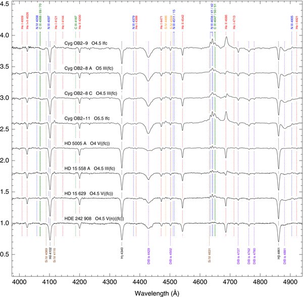
Figure 20. Spectrograms for normal stars.
Download figure:
Standard image High-resolution image
ζ Oph = HD 149 757. This object appears to have been ejected by a supernova explosion from Upper Scorpius (Hoogerwerf et al. 2000). It is a very fast rotator. Its revised Hipparcos distance with the new calibration is 112+3−3 pc (Maíz Apellániz et al. 2008), making it the nearest O star.
HD 167 659. Mason et al. (1998) give a companion at 008 but do not provide a Δm, so its effect is not included in the name. This star has been recently found out to be an SB1 (Gamen et al. 2008).
HD 165 319. This object was not present in version 1 of GOSC. In Maíz Apellániz (2004), it appeared as B0 Ia (Morgan et al. 1955).
HD 168 076 AB. This system has a separation of 0148 and a Δm of 1.7 mag in the H band. Sana et al. (2009) give a composite spectrum of O3.5 V ((f+)) + O7.5 V. See Figure 19 for a chart.
BD −13 4927. See Figure 19 for a chart.
BD −12 4979. This object was not present in version 1 of GOSC. See Figure 19 for a chart.
HD 173 010. This is an extremely luminous star. It might be classified Ia+ but for the absence of He ii λ4686 emission as in the LMC counterparts (Corti et al. 2009).
HD 173 783. The N iii spectrum is exceedingly strong but C iii is not abnormally weak.
HDE 344 783. This object was not present in version 1 of GOSC. See Figure 19 for a chart.
HDE 344 782. This object was not present in version 1 of GOSC. The spectrum includes two components (B and C) that are too dim to affect the spectral type. See Figure 19 for a chart.
HDE 344 784 A. Note that in Maíz Apellániz (2004) this object appears as BD +22 3782. See Figure 19 for a chart.
Cyg X-1 = V1357 Cyg = HDE 226 868. This system is the prototypical high-mass, black hole X-ray binary (Caballero-Nieves et al. 2009 and references therein).
HD 190 429 B. This object was not present in version 1 of GOSC. We were able to clearly separate the spectrum from that of A, located at a separation of 1959 with a Δm of 0.61 in the z band (Maíz Apellániz 2010).
HD 190 429 A. As already mentioned, we were able to separate the A and B spectra. Note that Mason et al. (1998) give an Ab component with a separation of 009 but with a large Δm, so its existence is not mentioned in the object name (i.e., it is A instead of AaAb).
HD 191 201 B. This object was not present in version 1 of GOSC.
HD 193 443 AB. Mason et al. (2009) give a separation between the A and B components of 013 with Δm = 0.3. We were unable to resolve the system. The C component is too dim to have an effect on spectrum (Mason et al. 1998).
HD 189 957. This is the standard for the newly introduced O9.7 III category.
HD 193 322 AaAb. Aa and Ab are separated by 0055 with a small Δm (Maíz Apellániz 2010; Mason et al. 2009) and are unresolved in our data. The B component is at a separation of 2719 and we were able to separate its spectrum from that of AaAb: it is an early-B star. This complex system was studied by McKibben et al. (1998), who found out that Aa is an SB1 with Ab in a 31 year period orbit around it. See Roberts et al. (2010) for a recent study of this system and the surrounding cluster, Collinder 419. The new Hipparcos calibration gives a revised distance of 708+255−145 pc (Maíz Apellániz et al. 2008).
V2185 Cyg = Schulte 50 = [MT91] 421. This object was not present in version 1 of GOSC. See Figure 19 for a chart.
Cyg OB2-22 A = Schulte 22 A = [MT91] 417 A. Cyg OB2-22 A and B are separated by 1521 with a Δm of 0.59 in the z band (Maíz Apellániz 2010). We were able to extract the individual spectra of A and B (see below for B). See also Walborn et al. (2002). This star has an extremely high spectroscopic/evolutionary mass and has not been resolved at high resolution, including HST/ACS (Maíz Apellániz 2010), HST/FGS, and Gemini AO (E. Nelan & D. Gies 2010, private communication), although a tighter structure cannot be ruled out. See Figure 19 for charts.
Cyg OB2-22 B = Schulte 22 B = [MT91] 417 B. Cyg OB2-22 B itself is a double system composed of Ba and Bb. Their separation is 0216 and their Δm is of 2.34 mag in the z band (Maíz Apellániz 2010), which is too large to have the effect of Bb included in the name of the object. See Figure 19 for charts.
NSV 13 148 = Schulte 24 = [MT91] 480. This object was not present in version 1 of GOSC. See Figure 19 for a chart.
Cyg OB2-8 B = Schulte 8 B = [MT91] 462. This object was not present in version 1 of GOSC. See Figure 19 for a chart.
Cyg OB2-8 D = Schulte 8 D = [MT91] 473. This object was not present in version 1 of GOSC. Note that the current version of the WDS catalog has Cyg OB2-8 C and D interchanged with respect to the most common usage. See Figure 19 for a chart.
Cyg OB2-7 = Schulte 7 [MT91] 457. See Figure 19 for a chart.
10 Lac = HD 214 680. The revised Hipparcos distance to this object with the new calibration is 542+77−59 pc (Maíz Apellániz et al. 2008).
HD 206 183. This object was not present in version 1 of GOSC. In Maíz Apellániz et al. (2004), a classification of B0 V was given.
HD 204 827 AaAb. This object was not present in version 1 of GOSC. Mason et al. (1998) give a separation of 012 and a Δm = 1.2 for the Aa + Ab system. B is more than 3 mag fainter. In Maíz Apellániz et al. (2004), a classification of B0.2 V was given.
HD 207 538. This object was not present in version 1 of GOSC. In Maíz Apellániz et al. (2004), a classification of B0.2 V was given but now is the standard for the newly introduced O9.7 IV category.
HD 207 198. Mason et al. (1998) give a companion with Δm = 3.5 at a separation of 183, so its effect does not modify the name.
HD 218 195 A. A B component at a separation of 0919 with a Δm of 2.56 in the z band was detected by Maíz Apellániz (2010). We were able to extract its spectrum independently of A and we obtained an early-B spectral type.
HD 5005 C. We obtained individual spectra for the four bright components in this system (A, B, C, and D) and we found all of them to be O stars. See Figure 19 for a chart.
HD 5005 B. We obtained individual spectra for the four bright components in this system (A, B, C, and D) and we found all of them to be O stars. This object was not present in version 1 of GOSC. The luminosity class from He ii λ4686/He i λ4713 conflicts with a very weak Si iv and probable extreme youth. See Figure 19 for a chart.
HD 5005 D. We obtained individual spectra for the four bright components in this system (A, B, C, and D) and we found all of them to be O stars. This object was not present in version 1 of GOSC. See Figure 19 for a chart.
BD +60 498. This object was not present in version 1 of GOSC. The luminosity class from He ii λ4686/He i λ4713 conflicts with a very weak Si iv and probable extreme youth. See Figure 19 for a chart.
BD +60 499. See Figure 19 for a chart.
BD +60 501. See Figure 19 for a chart.
HD 15 570. See Figure 19 for a chart.
HD 17 505 B. This object was not present in version 1 of GOSC. We were able to separate the spectrum from that of A, located at a separation of 2153 with a Δm of 1.75 in the z band (Maíz Apellániz 2010). See Figure 19 for charts.
HD 17 520 A. The A component is separated by only 0316 from the B component with a Δm of 0.67 mag in the z band (Maíz Apellániz 2010) but we were able to separate the two spectra. Hillwig et al. (2006) indicate that in the integrated A + B spectrum, the A component appears to be an SB1. In our spectra, we detect distinct velocity changes between the emission lines (which originate in B, see Section 3.2.5) and the absorption profile at different epochs, which supports the SB1 character for A. See Figure 19 for charts.
BD +60 586 A. See Figure 19 for a chart.
HD 15 137. McSwain et al. (2010) measure the SB1 orbit of this object and suggest that the unseen companion may be a neutron star or black hole.
HD 24 431. A B component is present at a separation of 0720 but its Δm of 2.9 in the z band (Maíz Apellániz 2010) indicates that it is too weak to have a significant effect in the optical spectrum.
ξ Per = Menkhib = HD 24 912. The revised Hipparcos distance to this object with the new calibration is 416+116−74 pc (Maíz Apellániz et al. 2008).
BD +39 1328. The spectrum of this star is rather anomalous: the neutralized He ii λ4686 indicates a high luminosity (as classified), but the Si iv and C iii absorptions are very weak, perhaps indicating a different origin of the He ii λ4686 behavior.
AE Aur = HD 34 078. This object appears to have been ejected from the Trapezium cluster (Hoogerwerf et al. 2000 and references therein).
HD 35 619. A B component is present at a separation of 2772 but its Δm of 2.88 in the z band (Maíz Apellániz 2010) indicates that it is too weak to have a significant effect in the optical spectrum.
BD +33 1025. This object was not present in version 1 of GOSC. See Figure 19 for a chart.
HDE 242 935 A. The A component is separated by 1081 from the B component with a Δm of 0.80 mag in the z band (Maíz Apellániz 2010). We were able to separate the two spectra and obtain an early-B type for the B component. See Figure 19 for charts.
HDE 242 926. See Figure 19 for a chart.
HD 93 521. This object is a non-radial pulsator (Rauw et al. 2008).
HD 44 811. See Figure 19 for a chart.
λ Ori A = HD 36 861. The A component is separated by 4342 from the B component with a Δm of 1.91 mag in the z band (Maíz Apellániz 2010). We were able to separate the two spectra and obtain an early-B type for the B component, which has a separate HD number (36 862). The revised Hipparcos distance to λ Ori A with new calibration is 361+89−60 pc (Maíz Apellániz et al. 2008).
15 Mon AaAb = S Mon AaAb = HD 47 839 AaAb. The three brightest components of this system are Aa, Ab, and B. 15 Mon B is at a separation of 2976 with respect to Aa and their Δm is of 3.23 mag in the z band (Maíz Apellániz 2010). We were able to spatially separate the B spectra in our data and confirm that it is of early-B type. Aa and Ab are much closer, with a separation of 0128 and a Δm of 1.43 in the z band, and we were unable to separate them. The Aa-Ab orbit is being followed with somewhat conflicting preliminary orbits at the present time: see Maíz Apellániz (2010) and references therein. The revised Hipparcos distance to the system with new calibration is 309+60−43 pc (Maíz Apellániz et al. 2008). The spectral type of this fundamental MK standard has been found to be apparently variable between O7 and O7.5 on an undetermined timescale, which is under investigation. Thus, it should be used with caution or not at all as a standard now. See Figure 19 for a chart.
HD 46 106. This object was not present in version 1 of GOSC. The luminosity class from He ii λ4686/He i λ4713 conflicts with a very weak Si iv and probable extreme youth.
HD 46 056 A. A B component at a separation of 10419 and a Δm of 2.78 mag in the z band (Maíz Apellániz 2010) was determined to be of early-B spectral type. Mahy et al. (2009) suggest that the broad lines of the A component are caused by rapid rotation.
ζ Ori B = HD 37 743. This object was not present in version 1 of GOSC. We were able to separate the B spectrum from that of A (=HD 37 742), located at a separation of 2424 and with a Δm of 2.26 mag in the z band. In Maíz Apellániz et al. (2004), it was given as an early-B giant but Garmany et al. (1982) listed it as O9.5 IV.
σ Ori AB = HD 37 468 AB. This system lies at the core of the well-studied σ Ori cluster (Caballero 2007; Sherry et al. 2008). The current separation between A and B is 0260; its orbit is followed by Turner et al. (2008). We were unable to spatially separate in our spectra the relatively low-Δm (1.57 in the z band) AB pair. See Figure 19 for charts.
θ1 Ori CaCb = HD 37 022 AB. This well-known object is the brightest star in the Trapezium and the main source of ionizing photons in the Orion nebula. In recent years, a bright companion (Δm = 1.3) has been detected at a small separation (tens of mas) and its orbit is currently being followed (Kraus et al. 2007, 2009; Patience et al. 2008). Ca is a magnetic oblique rotator with a period of 15.424 ± 0.001 days (Nazé et al. 2008b). The pair Ca-Cb is obviously unresolved in our spectra. See Figure 19 for a chart.
θ2 Ori A = HD 37 041. θ2 Ori A is the other O-type system in the Orion nebula. An Ab companion is spatially unresolved in our data (separation of 0396) but its Δm is too large (2.62 mag at the z band; Maíz Apellániz 2010) to have a significant effect in the observed spectra. The B and C components are farther away than 30'' and they have their own HD numbers (B is HD 37 042, C is HD 37 062; Mason et al. 1998). The revised Hipparcos distance with the new calibration is 520+201−103 pc (Maíz Apellániz et al. 2008). The luminosity class IV derived here from He ii λ4686/He i λ4713 is unlikely to represent a real luminosity effect in this probable zero-age main-sequence (ZAMS) star.
υ Ori = HD 36 512. This object was not present in version 1 of GOSC. Previously, it was a B0 V standard but now is the O9.7 V standard.
HD 52 533 A = BD −02 1885. There are several dim companions in the vicinity of HD 52 533 A but the brightest one is C, with a Δm of = 1.1 and a separation of 226 (Mason et al. 1998). We placed C on the slit and obtained a G spectral type for that component. See Figure 19 for a chart.
HD 57 682. A magnetic field has been discovered in this star (Grunhut et al. 2009). The spectral lines are extremely sharp and there are Balmer profile variations at high resolution very similar to those in the Of?p stars at earlier types.
4. SUMMARY
We have presented the first installment of a massive new survey of Galactic O-type spectra. On the basis of our extensive sample of high-quality, digital data in hand, we have reviewed the classification system and introduced several refinements designed to improve the accuracy and consistency of the spectral types. These include the routine use of luminosity class IV at spectral types O6–O8, and most importantly, a redefinition of the spectral-type criteria at late-O types so that they are uniform at all luminosity classes for a given subtype. As a consequence, some objects previously classified as B0 have moved into the newly defined O9.7 type for classes V through III, expanding the definition of the O spectral category. The list of standard spectra that define the system has been revised and expanded, including representatives of the new subcategories, although a few gaps in the two-dimensional grid remain to be filled from future observations. A new O-type classification atlas has likewise been provided. These developments, as well as enhanced convenience and accuracy of the digital classification in general, have been supported by a powerful new classification software tool that superimposes unknown with any standard spectrograms sequentially, along with capabilities to match the line widths and even double lines in spectroscopic binaries, iteratively with assumed parameters for the components. Attention to spatial resolution of close visual multiple systems has provided significantly improved information about their spectra, notably for HD 5005, HD 17 520, and HDE 242 935, in which the previous composite spectral types were misleading.
As expected from the substantial increases in the quantity, quality, and homogeneity of our sample, new members or characteristics of special categories, and even a new category (Ofc; Walborn et al. 2010a and above) of O-type spectra have been found. These also include the previously defined ON/OC, Onfp, Of?p, Oe, and SB categories, all of which have been discussed. Extensive notes and references have been given for many individual stars, both normal and peculiar; plots of all the spectrograms are provided, as well as charts for crowded regions. Analogous developments will be forthcoming in future installments of our program, particularly as we incorporate large numbers of fainter stars that have in general been less well observed previously than those presented here. Further astronomical and astrophysical discussion and applications of our results will be undertaken when the full sample is complete.
Support for this work was provided by (1) the Spanish Government Ministerio de Ciencia e Innovación through grant AYA2007-64052, the Ramón y Cajal Fellowship program, and FEDER funds; (2) the Junta de Andalucía grant P08-TIC-4075; (3) NASA through grants GO-10205, GO-10602, and GO-10898 from the Space Telescope Science Institute, which is operated by the Association of Universities for Research in Astronomy, Inc., under NASA contract NAS 5-26555; (4) the Dirección de Investigación de la Universidad de La Serena (DIULS PR09101); and (5) the ESO-Government of Chile Joint Committee Postdoctoral Grant. This research has made extensive use of (1) Aladin (Bonnarel et al. 2000); (2) the SIMBAD database, operated at CDS, Strasbourg, France; and (3) the Washington Double Star Catalog, maintained at the U.S. Naval Observatory (Mason et al. 2001).
Footnotes
-
*
The spectroscopic data in this article were gathered with three facilities: the 1.5 m telescope at the Observatorio de Sierra Nevada (OSN), the 3.5 m telescope at Calar Alto Observatory (CAHA), and the du Pont 2.5 m telescope at Las Campanas Observatory (LCO). Some of the supporting imaging data were obtained with the 2.2 m telescope at CAHA and the NASA/ESA Hubble Space Telescope (HST). The rest were retrieved from the DSS2 and Two Micron All Sky Survey (2MASS) surveys. The HST data were obtained at the Space Telescope Science Institute, which is operated by the Association of Universities for Research in Astronomy, Inc., under NASA contract NAS 5-26555.
-
12
-
13
As described in this paper, some stars previously classified as B0 V to III have been assigned new spectral types O9.7 V to III (previously, the O9.7 spectral type was defined only for luminosity classes II to Ia). Since we have only observed a small fraction of the stars with B < 8.0 previously classified as B0, it is possible that we have missed some O9.7 stars within that magnitude range.
-
14
-
15
Among the stars we are classifying as early-B there are some stars that had previously considered to be O stars, e.g., RY Sct and HD 194 280. The latter, the prototype late-OC supergiant, has been reclassified as BC0 Iab.
-
16
Hydrogen-rich WN stars appear to be relatively unevolved very massive stars (Crowther et al. 2010).
-
17
-
18
-
19
-
20
Note that from LCO it is possible to access declinations much farther north than δ = −20°, thus providing a large overlap region of the sky for the three observatories.
-
21
For some spectral types there are no northern standards in Maíz Apellániz et al. (2004).
-
22
Marxist Ghost Buster.
-
23
It is important to note that the printed atlas plots are necessarily very reduced. They must be enlarged online to reveal the full definition of the classification criteria, especially those involving weak lines. As previously mentioned, with v3.0 of GOSC we plan to make the data themselves available to the astronomical community.
-
24
Note that those values are only approximate: spectral classification is done by comparing data with standard spectra, such as those in Figure 12.
-
25
Classes IV and II and supergiant subclasses are not used at spectral types earlier than O6; thus, there is a range in the appearance of He ii λ4686 at class III for the earlier types.
-
26
The results for the third belt star,
 Ori = Alnilam, place it farther away but with a much larger uncertainty.
 -
27
Note that their D component is B here.