

Abstract
The surface warming response to carbon emissions is diagnosed using a suite of Earth system models, 9 CMIP6 and 7 CMIP5, following an annual 1% rise in atmospheric CO2 over 140 years. This surface warming response defines a climate metric, the Transient Climate Response to cumulative carbon Emissions (TCRE), which is important in estimating how much carbon may be emitted to avoid dangerous climate. The processes controlling these intermodel differences in the TCRE are revealed by defining the TCRE in terms of a product of three dependences: the surface warming dependence on radiative forcing (including the effects of physical climate feedbacks and planetary heat uptake), the radiative forcing dependence on changes in atmospheric carbon and the airborne fraction. Intermodel differences in the TCRE are mainly controlled by the thermal response involving the surface warming dependence on radiative forcing, which arise through large differences in physical climate feedbacks that are only partly compensated by smaller differences in ocean heat uptake. The other contributions to the TCRE from the radiative forcing and carbon responses are of comparable importance to the contribution from the thermal response on timescales of 50 years and longer for our subset of CMIP5 models and 100 years and longer for our subset of CMIP6 models. Hence, providing tighter constraints on how much carbon may be emitted based on the TCRE requires providing tighter bounds for estimates of the physical climate feedbacks, particularly from clouds, as well as to a lesser extent for the other contributions from the rate of ocean heat uptake, and the terrestrial and ocean cycling of carbon.
Export citation and abstract BibTeX RIS

Original content from this work may be used under the terms of the Creative Commons Attribution 4.0 license. Any further distribution of this work must maintain attribution to the author(s) and the title of the work, journal citation and DOI.
1. Introduction
Climate model projections reveal a simple emergent relationship that global-mean surface warming increases nearly linearly with the cumulative amount of carbon emitted since the pre-industrial era (Matthews et al 2009, Allen et al 2009, Zickfeld et al 2009, Gillett et al 2013, Collins et al 2013). This relationship is important as the sensitivity of warming to cumulative carbon emission dictates how much carbon may be released before reaching dangerous climate (Meinshausen et al 2009, Zickfeld et al 2009, Matthews et al 2012). This constraint provides a basis for the Paris climate agreement (Rogelj et al 2016) where limits are provided for how much carbon may be emitted to avoid exceeding 1.5°C or 2°C warming (Millar et al 2017, Goodwin et al 2018).
While climate model projections reveal this near linear relationship between surface warming and cumulative carbon emissions during emissions, the precise slope of this surface warming relationship differs among individual climate models (Gillett et al 2013, Williams et al 2017); such as illustrated in figure 1 for a suite of 9 CMIP6 and 7 CMIP5 Earth system models following a 1% annual increase in atmospheric CO2. This slope varies from 1.10 to 2.35 K EgC−1 within the 9 CMIP6 models and from 1.32 to to 2.16 K EgC−1 within the 7 CMIP5 models (table 1). The intermodel differences in the surface warming response lead to a wide range in these model-based estimates of the maximum permitted carbon emission to avoid a particular warming target. As an example, for a 2°C warming target, the maximum permitted emissions extend from 760 PgC to 1690 PgC for the 9 CMIP6 models and 830 to 1460 PgC for the 7 CMIP5 model integrations (table 1). Hence, there is a need to understand the reasons for these intermodel differences in the rate at which surface warming increases given a carbon emission, both for the latest set of CMIP6 models and their differences with CMIP5 models (MacDougall et al 2017, Williams et al 2017, Jones and Friedlingstein 2020).
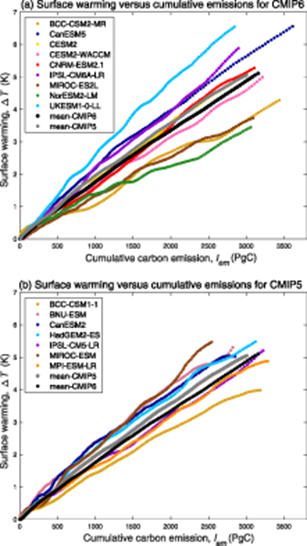
Figure 1. Change in global-mean surface air temperature, ΔT(t) in K, versus change in cumulative carbon emissions, Iem in PgC, since the pre-industrial for (a) 9 CMIP6 models and (b) 7 CMIP5 models, assuming an annual 1% increase in atmospheric CO2 and integrated for 140 years.
Download figure:
Standard image High-resolution imageTable 1. List of 9 CMIP6 and 7 CMIP5 Earth system models diagnosed in this study following an 1% annual increase in atmospheric CO2 together with the TCRE over years 120 to 140, and the cumulative carbon emission when 2°C warming is reached.
| TCRE | Carbon emission (PgC) | |||||
|---|---|---|---|---|---|---|
| Model Name | (K EgC−1) | at 2°C warming | Reference | |||
| CMIP6: | ||||||
| BCC-CSM2-MR | 1.22 | 1550 | (Wu et al 2019) | |||
| CanESM5 | 1.86 | 921 | (Swart et al 2019) | |||
| CESM2 | 1.72 | 1120 | (Danabasoglu et al 2020) | |||
| CESM2-WACCM | 1.55 | 1180 | ||||
| CNRM-ESM2-1 | 1.76 | 1250 | (Seferian et al 2019) | |||
| IPSL-CM6A-LR | 1.99 | 938 | (Boucher et al 2020) | |||
| MIROC-ES2L | 1.22 | 1490 | (Hajima et al 2019) | |||
| NorESM2-LM | 1.10 | 1688 | (Seland et al 2020, in prep) | |||
| UKESM1-0-LL | 2.35 | 758 | (Sellar et al 2019)\\ CMIP5: | |||
| BCC-CSM1-1 | 1.32 | 1457 | (Wu et al 2013) | |||
| BNU-ESM | 1.92 | 852 | (Ji et al 2014) | |||
| CanESM2 | 1.88 | 833 | (Arora et al 2011) | |||
| HadGEM2-ES | 1.82 | 926 | (Collins et al 2011) | |||
| IPSL-CM5A-LR | 1.58 | 1192 | (Dufresne et al 2013) | |||
| MIROC-ESM | 2.16 | 935 | (Watanabe et al 2011) | |||
| MPI-ESM-LR | 1.55 | 1287 | (Ilyina et al 2013) |
This ratio of surface warming to cumulative carbon emissions is used to define a climate index, the Transient Climate Response to cumulative carbon Emissions (TCRE), which is relevant on decadal and centennial timescales when there are carbon emissions (Matthews et al 2009, Gillett et al 2013, Collins et al 2013, MacDougall 2016, Williams et al 2016, Matthews et al 2018, Katavouta et al 2018). Our aim is to exploit theory to understand how this surface warming relationship in climate model projections is controlled by physical climate feedbacks, heat uptake, saturation of radiative forcing and carbon cycling.
In this study, the sensitivity of this surface warming to cumulative carbon emissions is examined using diagnostics for a suite of 9 CMIP6 and 7 CMIP5 Earth system models. In section 2, different identities for the TCRE are set out, either related to changes in temperature, the amount of atmospheric carbon and emitted carbon (Matthews et al 2009) or related to changes in temperature, radiative forcing and emitted carbon (Goodwin et al 2015, Williams et al 2016, Williams et al 2017), or variants of these identities combined together (Ehlert et al 2017, Katavouta et al 2018). Our physically-motivated analysis is complemented by a related TCRE analysis based on carbon-cycle feedbacks by Jones and Friedlingstein (2020). In section 3, diagnostics on subsets of the CMIP6 and CMIP5 Earth system models are applied to identities for the TCRE, providing a mechanistic view of how intermodel differences in the TCRE are controlled by physical climate feedbacks, planetary heat uptake, the dependence of radiative forcing on atmospheric CO2 and the airborne fraction involving the carbon cycle. Finally, in section 4, the implications of the study are summarised.
2. Theory
The Transient Climate Response to Emissions (TCRE) measures the sensitivity of surface warming to cumulative carbon emissions, which is defined by the change in global-mean surface air temperature, ΔT(t) in K, relative to the pre-industrial divided by the cumulative carbon emission, Iem(t) in EgC, such that
The TCRE is often viewed in terms of a product of two terms, the change in global-mean air temperature divided by the change in the atmospheric carbon inventory, ΔIatmos(t), and the change in the atmospheric carbon inventory divided by the cumulative carbon emission,  (Matthews et al 2009, Solomon et al 2009, Gillett et al 2013, MacDougall 2016), such that
where ΔT(t)/ΔIatmos(t) is related to the Transient Climate Response, defined by the temperature change at the time of doubling of atmospheric CO2 (Matthews et al 2009), and  defines the airborne fraction.
Alternatively, the TCRE in (2) may be linked to an identity involving a thermal response to radiative forcing, defined by the change in temperature divided by the change in radiative forcing, ΔF, and a radiative forcing response to carbon emissions, defined by the change in radiative forcing divided by the cumulative carbon emissions (Goodwin et al 2015, Williams et al 2016, Williams et al 2017), such that
which may be extended by rewriting the radiative forcing dependence to carbon emissions in terms of the radiative forcing dependence on atmospheric CO2 and the airborne fraction (Ehlert et al 2017, Katavouta et al 2018),
Each of these identities for the TCRE have different potential merits: the first identity (2) provides a clearer connection to changes in carbon cycling via the airborne fraction, while the second identity (3) provides a clearer connection to the thermal processes of climate feedbacks and ocean heat uptake, and to the radiative forcing that depends upon the change in the logarithm of atmospheric CO2. Here, we focus on the combined identity for the TCRE (4), including the effects of the thermal response, the radiative forcing and the airborne fraction.
2.1. Dependence of surface warming on radiative forcing
The increase in radiative forcing, ΔF(t), drives an increase in planetary heat uptake, N(t), plus a radiative response, ΔR(t), which is assumed to be equivalent to the product of the increase in global-mean surface air temperature, ΔT(t), and the climate feedback parameter, λ(t) (Gregory et al 2004, Knutti and Hegerl 2008, Andrews et al 2012, Forster et al 2013) by

where N(t) is the planetary heat flux into the climate system, which is dominated by the heat uptake by the ocean (Church et al 2011), and ΔF(t) is defined as positive into the ocean.
The dependence of surface warming on radiative forcing, ΔT(t)/ΔF(t), in (3) is then directly connected to the product of the inverse of the climate feedback, λ(t)−1, and the planetary heat uptake divided by the radiative forcing, N(t)/ΔF(t),
where (1 − N(t)/ΔF(t)) represents the fraction of the radiative forcing that warms the surface, rather than the ocean interior.
2.2. Dependence of radiative forcing from atmospheric CO2 on carbon emissions
The dependence of radiative forcing on cumulative carbon emissions, ΔF(t)/Iem(t), in (3) may be expressed in terms of changes in the radiative forcing on changes in atmospheric CO2, ΔF(t)/ΔIatmos(t), and the airborne fraction,  (Ehlert et al 2017),
The airborne fraction,  , is related to the changes in the oceanborne and landborne fractions (Jones et al 2013),
where the changes in the ocean and terrestrial inventories are denoted by ΔIocean(t) and ΔIter(t) respectively.
The sensitivity of the radiative forcing on atmospheric CO2, ΔF(t)/ΔIatmos(t), saturates with increasing atmospheric CO2, with the radiative forcing represented by a logarithmic dependence,

where a is a radiative forcing coefficient for CO2 (Myhre et al 1998) and t0 is the time of the pre-industrial. During emissions, the decrease in the sensitivity of the radiative forcing on atmospheric CO2, ΔF(t)/ΔIatmos(t), may equivalently be viewed in terms of the ocean acidifying with increasing atmospheric CO2 and decreasing the amount of saturated carbon that the ocean can hold (Katavouta et al 2018).
Next we apply these theoretical relations (3) to (9) to understand how the TCRE is controlled.
3. Methods
3.1. Models
Our analyses are applied to 9 CMIP6 and 7 CMIP5 models (table 1), which have been forced by an annual 1% rise in atmospheric CO2 for 140 years starting from a pre-industrial control, following the 1pctCO2 experimental protocol (Eyring et al 2016). All the thermal and carbon diagnostics are performed on the forced model response with the unforced pre-industrial control (piControl) subtracted off to minimise model drift.
3.2. Carbon diagnostics
The Earth system models couple the carbon cycle and climate together through sources and sinks of CO2 being affected by atmospheric CO2 and the change in climate (Ciais et al 2014). The sum of the changes in the atmospheric, ocean and terrestrial inventories of carbon balance the implied cumulative carbon emission, Iem(t) in PgC,

where the inventory changes are evaluated from the time integral of the air-sea and air-land carbon fluxes. The model mean for the cumulative carbon emission, Iem(t), is 2790 and 2700 PgC for years 120 to 140 for the 9 CMIP6 and the 7 CMIP5 models respectively (table 2). There are differences in the cumulative carbon emission in each of the individual Earth system models from differences in their terrestrial and ocean cycling and uptake of carbon (Arora et al 2019) (figure 2(a)).
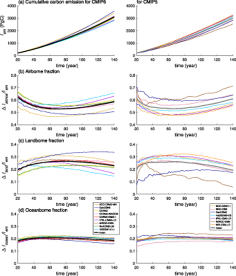
Figure 2. Evolution of the carbon budget over 140 years for 9 CMIP6 (left panels) and 7 CMIP5 (right panels) Earth system models together with their model mean (thick black and grey lines): (a) cumulative carbon emission, Iem in PgC; (b) airborne fraction,  ; (c) landborne fraction,
  ; and (d) oceanborne fraction,
  .
.
Download figure:
Standard image High-resolution imageTable 2. Model mean, intermodel standard deviation and coefficient of variation for the thermal and carbon variables for years 120 to 140 for the 9 CMIP6 and 7 CMIP5 Earth system models following a 1% annual increase in atmospheric CO2. The coefficient of variation is defined by the intermodel standard deviation divided by the model mean, evaluated at the same time. The individual model responses are provided in table S1.
| Variable: | ΔT | F | N | λ | N/F | Iem |  |
 |
 |
|||||||||
|---|---|---|---|---|---|---|---|---|---|---|---|---|---|---|---|---|---|---|
| Units: | K | W m−2 | W m−2 | (W m−2)K−1 | PgC | |||||||||||||
| CMIP6 | ||||||||||||||||||
mean,  |
4.55 | 7.27 | 2.42 | 1.16 | 0.33 | 2787 | 0.57 | 0.19 | 0.24 | |||||||||
| std, σx | 1.04 | 0.45 | 0.35 | 0.45 | 0.05 | 213 | 0.04 | 0.02 | 0.05 | |||||||||
 |
0.23 | 0.06 | 0.14 | 0.39 | 0.16 | 0.08 | 0.08 | 0.08 | 0.22\\ CMIP5 | |||||||||
mean,  |
4.66 | 7.21 | 2.28 | 1.05 | 0.32 | 2702 | 0.59 | 0.20 | 0.21 | |||||||||
| std, σx | 0.42 | 0.98 | 0.41 | 0.21 | 0.05 | 249 | 0.06 | 0.02 | 0.06 | |||||||||
 |
0.09 | 0.14 | 0.18 | 0.20 | 0.16 | 0.09 | 0.10 | 0.09 | 0.31 |
The airborne fraction,  , initially falls to a minimum between years 50 and 80, and then increases in time reaching model means of 0.57 for the 9 CMIP6 models and 0.59 for the 7 CMIP5 models for years 120 to 140 (figure 2(b), table 2). This response is a consequence of the landborne fraction,
  , increasing in time to a maximum over a wide range from years 30 to 120, and then decreasing (figure 2(c)), as well as from the oceanborne fraction,
  , increasing to a maximum around year 50 and then slightly decreasing (figure 2(d)). The response of the CMIP6 models is broadly similar to that of the CMIP5 models, although there is a greater range in the intermodel differences in the airborne, landborne and oceanborne fractions for CMIP5 (tables 2 and S1 (stacks.iop.org/ERL/15/0940c1/mmedia)).
3.3. Thermal diagnostics
For the thermal analyses, the planetary heat uptake, N(t), is provided from 1pctCO2 model output, but the radiative forcing, ΔF(t), radiative response, ΔR(t), and the climate feedback parameter, λ(t), need to be diagnosed. The effective radiative forcing, ΔF(t), is calculated using the logarithmic dependence in (9) with the radiative forcing coefficient  . The effective forcing due to a quadrupling of atmospheric CO2,
  , is diagnosed from the abrupt-4xCO2 simulations using the y-intercept of a regression fit for N(t) versus ΔT(t) (Gregory et al 2004). To account for curvature in the N(t) versus ΔT(t) relationship (Andrews et al 2015), only the first twenty years of data are used to calculate the fits.
The regression-based estimate of  yields an incorrect value for the CNRM-ESM2.1 model, because in this model simulation for abrupt-4xCO2 the quadrupling of CO2 concentration takes about 15 years, rather than being instantaneous (see the discussion in Smith et al (2020)). Therefore for this model only, the forcing is estimated as the difference in N(t) between two fixed sea surface temperature simulations, piClim-4xCO2 and piClim-control (table 2 in Smith et al (2020)).
The radiative response, ΔR(t), is next diagnosed from ΔF(t)−N(t). The time-varying climate feedback parameter, λ(t), is then diagnosed from the least-squares regression slope of ΔR(t) against ΔT(t) (Gregory and Forster 2008), where the regression is calculated from the start of the time series to year t. For example, λ(t) for year 70 is based on the regression over the first 70 years, while λ(t) for year 140 is based on the regression over the entire 140 years.
The diagnostics for ΔR(t), ΔF(t), N(t) and ΔT(t) are smoothed to remove interannual variability using a moving average filter with a 10 year window.
The physical feedback parameter, λ(t), is further decomposed into contributions from the Planck feedback, the lapse rate, relative humidity, surface albedo and cloud feedbacks,

where the subscripts identify each component. The radiative impact of water vapour is separated into two contributions: changes at constant relative humidity, counted as part of the temperature-driven response, and a residual contribution due to changes in relative humidity (Held and Shell 2012). The radiative decomposition is performed using CAM5 radiative kernels (Pendergrass et al 2017, Soden et al 2008).
In these Earth system models integrated under a 1% annual increase in atmospheric CO2 scenario, the radiative forcing ΔF(t) is typically 7.3 W m−2 for years 120 to 140 (figure 3(a)), which drives an increase in planetary heat uptake, N(t), of typically 2.4 W m−2 and a radiative response, ΔR(t), of 4.9 W m−2 (figure 3(b) and (c), table 2). The climate feedback parameter, λ(t), varies across the models from 0.7 to 2.5 W m−2 K−1 with a model mean of 1.2 W m−2 K−1 (figure 3(d)). There is a larger intermodel range in the radiative response and climate feedback parameter for the 9 CMIP6 models compared with for the 7 CMIP5 models (figure 3(c) and (d)), reaching twice the normalised spread based upon the ratio of the standard deviation over the model mean (table 2).
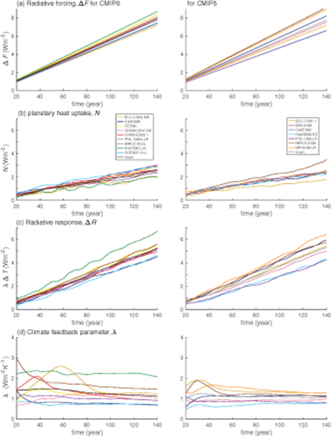
Figure 3. Evolution of the radiative and heat budget over 140 years for 9 CMIP6 (left panels) and 7 CMIP5 (right panels) Earth system models together with their model means (thick black and grey lines): (a) radiative forcing, ΔF in W m−2, which drives an increase in (b) planetary heat uptake, N in W m−2 and (c) a radiative response, ΔR in W m−2, together with (d) the climate feedback parameter, λ = ΔR/ΔT in W m−2K−1.
Download figure:
Standard image High-resolution image4. Diagnostics of the TCRE
The response of the Earth system models is now assessed in terms of the TCRE and its relationship to thermal, radiative forcing and carbon-cycle responses of the climate system.
4.1. Evolution of the TCRE
The TCRE only slightly varies in time over the 140 years for most of the Earth system models (figure 4(a)), although sometimes there is a slight decrease in time. The evolution of the TCRE is usually viewed in terms of the product of the ratio of the surface warming and the change in atmospheric carbon, ΔT/ΔIatmos, and the airborne fraction,  , in (2) (Matthews et al 2009), as illustrated in figures 4(b) and (c); this expression may be equivalently written in terms of the product of a climate sensitivity and carbon feedback parameters (Jones and Friedlingstein 2020).
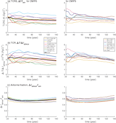
Figure 4. Evolution of the TCRE, surface warming dependence on atmospheric carbon and airborne fraction for 9 CMIP6 (left panels) and 7 CMIP5 (right panels) Earth system models together with their model means (thick black and grey lines): (a) the TCRE from the dependence of surface warming on cumulative carbon emissions, ΔT/Iem in K EgC−1; (b) the Transient Climate Response (TCR) from the dependence of surface warming on atmospheric carbon, ΔT/ΔIatmos in K (EgC)−1; and (c) the airborne fraction,  .
.
Download figure:
Standard image High-resolution imageFor the 9 CMIP6 models, the TCRE contribution from the ratio of the surface warming and the change in atmospheric carbon, ΔT/ΔIatmos, typically involves a slight decline, while the airborne fraction,  , involves an initial decline and then a slight increase (figures 4(b) and (c), grey line). There is a broadly similar response for the 7 CMIP5 models, but slightly modified by ΔT/ΔIatmos decreasing after typically year 40 and with a larger intermodel spread in the airborne fraction. While the near constancy of the TCRE is clear in these diagnostics, the control of the TCRE for different individual Earth system models is not particularly revealing using this identity (figure 4, table S1).
Instead we advocate that the TCRE may be interpreted in terms of a product of the thermal response, involving the surface warming dependence on radiative forcing, ΔT/ΔF, and a radiative forcing response, involving the dependence of radiative forcing on carbon emissions, ΔF/Iem in (3) (Williams et al 2016, Williams et al 2017), as illustrated in figure 5.
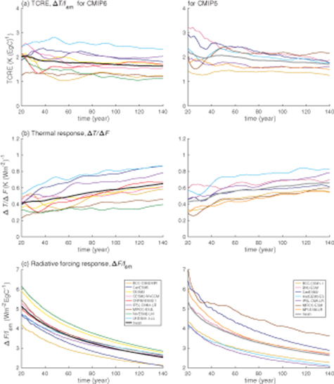
Figure 5. Evolution of the TCRE and its components for 9 CMIP6 (left panels) and 7 CMIP5 (right panels) Earth system models together with their model means (thick black and grey lines): (a) the TCRE from the dependence of surface warming on cumulative carbon emissions, ΔT/Iem in K EgC−1; (b) the thermal response from the dependence of surface warming on radiative forcing, ΔT/ΔF in K (W m−2)−1; and (c) the dependence of radiative forcing on cumulative carbon emissions, ΔF/Iem in (W m−2) EgC−1.
Download figure:
Standard image High-resolution imageUsing this identity, the thermal response, ΔT/ΔF, is revealed to increase in time for all the models (figure 5(b)), while the radiative forcing response, ΔF/Iem, decreases in time (figure 5(c)). There is a broadly similar dependence in both the subsets of the CMIP6 and CMIP5 models. The intermodel spread is greater for the thermal response, ΔT/ΔF, and is instead smaller for the radiative forcing response, ΔF/Iem for the 9 CMIP6 models relative to the 7 CMIP5 models (figure 5(b) and (c); tables 3 and S2).
Table 3. Model mean, intermodel standard deviation and coefficient of variation for the TCRE and its components for years 120 to 140 for the 9 CMIP6 and 7 CMIP5 Earth system models following a 1% annual increase in atmospheric CO2. The coefficient of variation is defined by the intermodel standard deviation divided by the model mean, evaluated at the same time. The individual model responses are provided in table S2.
| Variable: | TCRE | ΔT/ΔIatmos | ΔT/ΔF | ΔF/Iem | λ−1 | (1−N/ | ΔF/ΔIatmos |  |
|---|---|---|---|---|---|---|---|---|
| Units: | K EgC−1 | K EgC−1 | K (W m |
(W m−2) (EgC)−1 | K (W m |
ΔF) | (W m−2) (EgC)−1 | Iem |
| CMIP6 | ||||||||
mean,  |
1.64 | 2.87 | 0.63 | 2.63 | 0.96 | 0.67 | 4.59 | 0.57 |
| std, σx | 0.41 | 0.65 | 0.17 | 0.27 | 0.31 | 0.05 | 0.30 | 0.04 |
 |
0.25 | 0.23 | 0.26 | 0.10 | 0.32 | 0.08 | 0.06 | 0.08 |
| CMIP5 | ||||||||
mean,  |
1.75 | 2.94 | 0.66 | 2.71 | 0.99 | 0.68 | 4.55 | 0.59 |
| std, σx | 0.28 | 0.27 | 0.10 | 0.56 | 0.21 | 0.05 | 0.62 | 0.06 |
 |
0.16 | 0.09 | 0.16 | 0.21 | 0.21 | 0.07 | 0.14 | 0.10 |
Hence, the near constancy of the TCRE is a consequence of nearly compensating contributions: a strengthening in the thermal response, ΔT/ΔF, offsetting a weakening in the radiative forcing response, ΔF/Iem.
4.2. Evolution of the components of the TCRE
The strengthening in the thermal response given by the surface warming dependence on radiative forcing, ΔT/ΔF (figure 6(a)), from (6) is due to two reinforcing contributions: (i) a weakening in the climate feedback parameter, λ, and (ii) an increase in the fraction of radiative forcing used to warm the surface, (1 − N(t)/ΔF(t)) (figure 6(b) and (c)). The decrease in λ over time is a well-documented feature of the response of coupled climate models to CO2 forcing (Andrews et al 2015), resulting from sea surface warming patterns evolving in time (Armour et al 2013, Rugenstein et al 2016, Ceppi and Gregory 2017, Andrews and Webb 2018). The reducing fraction of radiative forcing taken up by the ocean interior is also well reported (Solomon et al 2009, Goodwin et al 2015, Williams et al 2016, Williams et al 2017). This thermal response is similar in pattern for both the CMIP6 and CMIP5 models. There is though a greater intermodel spread in these thermal responses and their contributions from λ−1 for the 9 CMIP6 models relative to the 7 CMIP5 models (table 3).
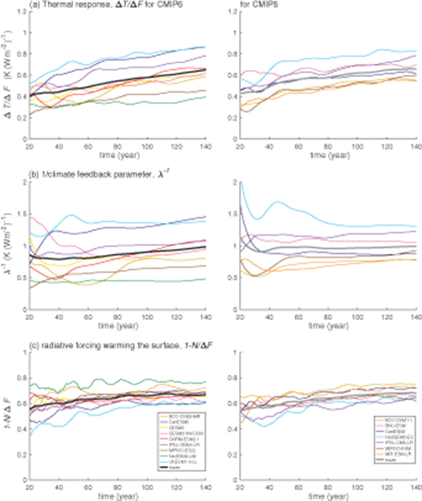
Figure 6. Evolution of (a) the thermal response from the dependence of surface warming on radiative forcing, ΔT/ΔF in K (W m−2)−1; (b) 1/climate feedback parameter, λ−1 in K (W m−2)−1; and (c) the fraction of radiative forcing that warms the surface, (1 − N/ΔF), for 9 CMIP6 (left panels) and 7 CMIP5 (right panels) Earth system models together with their model means (thick black and grey lines).
Download figure:
Standard image High-resolution imageThe weakening in the radiative forcing response given by the radiative forcing dependence on cumulative carbon emissions, ΔF/Iem (figure 7(a)), from (7) is mainly due to a weakening in the radiative forcing dependence on atmospheric carbon, ΔF/ΔIatmos, from a saturating effect (Myhre et al 1998) together with smaller contributions from the changes in the airborne fraction (Matthews et al 2009) (figure 7(b) and (c)). This response is also explained in terms of how far the ocean is from a carbon equilibrium with the atmosphere (Goodwin et al 2015, Williams et al 2017, Katavouta et al 2018). This radiative forcing response is similar in pattern for both the CMIP6 and CMIP5 models. There is though a smaller intermodel spread in both the radiative forcing dependence on atmospheric carbon and the changes in the airborne fraction responses for the 9 CMIP6 models relative to the 7 CMIP5 models (table 3).
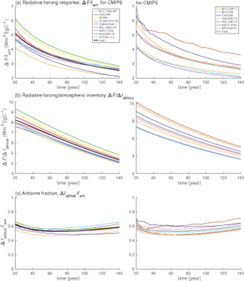
Figure 7. Evolution of (a) the dependence of radiative forcing on cumulative carbon emissions, ΔF/Iem in W m−2 EgC−1; (b) the ratio of the radiative forcing and the change in the atmospheric carbon inventory, ΔF/ΔIatmos in W m−2 EgC−1; and (c) the airborne fraction,  , for 9 CMIP6 (left panels) and 7 CMIP5 (right panels) Earth system models together with their model means (thick black and grey lines).
Download figure:
Standard image High-resolution image4.3. Intermodel spread for the TCRE
The normalised spread for the separate sets of 9 CMIP6 and 7 CMIP5 models are next assessed by diagnosing the coefficient of variation (also called the relative standard deviation) given by the intermodel standard deviation for each variable and dividing by the multi-model mean, all evaluated at the same time (Williams et al 2017, Katavouta et al 2019). The normalised spreads for the TCRE for years 120 to 140 are 0.25 and 0.16 for the subsets of 9 CMIP6 and 7 CMIP5 models respectively (figure 8(a), tables 3 and S2).
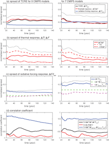
Figure 8. Evolution of the normalised spread of the TCRE and its components for 9 CMIP6 models (left column) and 7 CMIP5 models (right column), given by the coefficient of variation (from the intermodel standard deviation divided by the model mean): (a) the TCRE, ΔT/Iem (thick black line), and its components for the thermal response, ΔT/ΔF (red line) and the radiative forcing response, ΔF/Iem (blue line), together with the expected variation of the TCRE (grey line) if each of the contributions operate independently of each other; (b) the thermal response given by the dependence of surface warming on radiative forcing, ΔT/ΔF (red line), 1/climate feedback, λ−1 (dashed red line) and the fraction of the radiative forcing warming the ocean interior, ΔN/F (red dot-dash line) together with the expected variation of the ΔT/ΔF (grey line); and (c) the dependence of radiative forcing on cumulative carbon emissions, ΔF/Iem (blue line), the ratio of the radiative forcing and the change in the atmospheric carbon inventory, ΔF/ΔIatmos (green dashed line) and the airborne fraction,  (purple dashed line) together with the expected variation of the ΔF/Iem (grey line). In addition, (d) shows the correlation coefficient for each of the components included in (a) to (c).
Download figure:
Standard image High-resolution imageFor the CMIP6 subset of models, there is a larger normalised spread for ΔT/ΔF of 0.26 and a smaller normalised spread for ΔF/Iem of 0.10. Instead for the CMIP5 subset of models, there is the opposing response with a smaller normalised spread for ΔT/ΔF of 0.16 and larger normalised spread for ΔF/Iem of 0.21 (figure 8(a), table 3). Hence, for years 120 to 140, the intermodel spread for the TCRE is being controlled more strongly by the thermal response for the 9 CMIP6 models, but instead more strongly by the radiative and carbon responses for the 7 CMIP5 models.
If the normalised spread for each thermal and radiative forcing responses, ΔT/ΔF, and ΔF/Iem, were assumed to be independent of each other and combined in the same manner as random errors, then the normalised spread for the TCRE would be comparable to the square root of the sum of the squared contributions making up the TCRE in (3) (figure 8(a), grey line). This estimate of the normalised spread from the sum of these two contributions, ΔT/ΔF and ΔF/Iem, is always larger than the actual normalised spread for the TCRE. This inference of partial compensation is supported by the two contributions, ΔT/ΔF and ΔF/Iem, being negatively correlated to each other with a correlation coefficient value of typically -0.5 (figure 8(d), black line).
4.4. Uncertainties in ΔT/ΔF and ΔF/Iem
The normalised spread for the thermal response, ΔT/ΔF, ranges typically from 0.2 to 0.3 for both the CMIP6 and CMIP5 models (figure 8(b)), but the normalised spread becomes larger for the CMIP6 models than the CMIP5 models by years 120 to 140 (table 3). The normalised spread of ΔT/ΔF in both the CMIP6 and CMIP5 models is dominated by the contribution of the inverse of the climate feedback, λ−1, rather than from the fraction of the radiative forcing used to warm the surface, 1 − N/ΔF, where N is effectively the ocean heat uptake, based upon (6). This response does differ though between these subsets of CMIP6 and CMIP5 models with a larger spread for the λ−1 contribution for CMIP6 for years 120 to 140 (table 3).
While the intermodel spread in λ−1 is more important than that in ocean heat uptake, N, there is a strong partial compensation in the changes in λ−1, and the fraction of the radiative forcing used to warm the ocean interior, N/ΔF, with a correlation coefficient of typically -0.9 (figure 8(d), red line). Hence for a given radiative forcing, a larger physical climate feedback is associated with less ocean heat uptake, whereas a smaller physical climate feedback is associated with more ocean heat uptake.
The normalised spread for the radiative forcing response, ΔF/Iem, is typically 0.1 for the 9 CMIP6 models and 0.2 for the 7 CMIP5 models (figure 8(c), table 3). This smaller normalised spread for CMIP6 is through smaller reinforcing contributions from the dependence of the radiative forcing on atmospheric carbon, ΔF/ΔIatmos, and the airborne fraction,  based upon (7); both terms have a weak positive correlation to each other of typically 0.5 or less (figure 8(d), blue line). The intermodel differences in the airborne fraction are themselves more dominated by the landborne fraction (figures 2(b)–(d)); the intermodel spread for the landborne fraction is a factor of 2 or 3 larger than that for the oceanborne faction for CMIP6 and CMIP5 respectively (tables 2 and S1).
4.5. Effects of physical climate feedbacks
A dominant cause of intermodel differences in the TCRE is from the thermal response, which is itself mainly controlled by intermodel differences in the physical climate feedback for both the 9 CMIP6 and 7 CMIP5 models. The overall radiative response and climate feedback parameter is positive, acting to cool the surface (figure 9(a)).
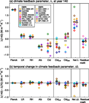
Figure 9. (a) Climate feedback parameter λ, in W m−2 K−1, diagnosed using a regression over years 1 to 140 of the 1% annual increase in atmospheric CO2 simulations of 9 CMIP6 (diamonds) and 7 CMIP5 models (circles), decomposed into contributions from the Planck feedback, changes in the lapse rate (LR), relative humidity (RH), surface albedo (Alb) and clouds (Cld). The cloud term is further separated into longwave (LW) and shortwave (SW) contributions. The sum of the climate feedbacks is given by the net feedback (Net). The residual misfit is the difference between the net feedback and the sum of the kernel-decomposed feedbacks, reflecting inaccuracies in the kernel method. (b) Time evolution of λ, calculated as the difference between λ(140) and λ(70), where λ(70) is diagnosed using a regression over years 1 to 70 of the experiment and λ(140) over years 1 to 140. The sign convention is such that positive values for λ in (5) imply a negative physical feedback acting to oppose surface warming.
Download figure:
Standard image High-resolution imageThe dominant contribution to the physical climate feedback, λ, in (11) is the Planck feedback (figure 9(a)) acting to cool the surface (with a positive λ in our sign convention), which is reinforced by smaller positive contributions from the lapse rate and relative humidity. There are negative contributions from the albedo and generally from clouds, both acting to increase surface warming. The intermodel spread in λ is dominated by intermodel differences in the shortwave and longwave effects of clouds with the net effect of clouds ranging from strongly negative (acting to enhance surface warming) to weakly positive (Ceppi et al 2017).
The analyses for the contribution to the feedback parameter, λ, between the sets of CMIP6 and CMIP5 models vary from being almost identical to very similar for the Planck feedback, the lapse rate and relative humidity contributions (figure 9(a)). There is a narrower spread for the albedo contribution for CMIP6 relative to CMIP5. However, there is a larger spread for the longwave and shortwave contributions from clouds for CMIP6 relative to CMIP5, which leads to the overall net climate feedback parameter having a larger positive range for CMIP6 (figure 9(a), tables 2 and S1).
The feedback parameter, λ, does evolve in time, consistent with figure 6(b), becoming smaller in magnitude, mainly due to the shortwave cloud contribution becoming more negative and acting to enhance surface warming (figure 9(b)). These analyses are in agreement with diagnostics of more extensive sets of CMIP5 and CMIP6 models (Andrews et al 2015, Ceppi and Gregory 2017, Ceppi et al 2017, Zelinka et al 2020).
4.6. Comparison of the drivers of the TCRE between CMIP5 and CMIP6
The spread in the TCRE is now presented in a normalised fashion for each set of 9 CMIP6 and 7 CMIP5 models, where each model response is normalised by dividing by the model mean for years 120 to 140 (figure 10, left column). There is a slightly larger normalised spread for this subset of 9 CMIP6 compared with the subset of 7 CMIP5 models. This difference is probably a consequence of the choice and number of the models analysed, since other studies do not find a significant difference in the TCRE for CMIP5 and CMIP6 (Arora et al 2019, Jones and Friedlingstein 2020).
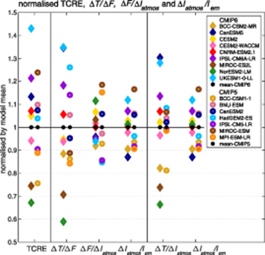
Figure 10. Intermodel normalised spread for the TCRE and its components for 9 CMIP6 (diamonds) and 7 CMIP5 models (circles) over years 120 to 140 including the thermal response from the dependence of surface warming on radiative forcing, ΔT/ΔF, the radiative forcing dependence on the change in atmospheric carbon, ΔF/ΔIatmos, and the airborne fraction,  . Each of the individual model responses are normalised by the relevant model mean for either CMIP6 or CMIP5 over years 120 to 140. For comparison, the normalised spread is also shown for the TCR, ΔT/ΔIatmos, and the airborne fraction,
  .
.
Download figure:
Standard image High-resolution image
There are robust differences in the controls of the intermodel differences in the TCRE as revealed by separating the TCRE into a thermal response involving the dependence of surface warming on radiative forcing, ΔT/ΔF, the dependence of the radiative forcing on atmospheric CO2, ΔF/ΔIatmos, and the airborne fraction,  (figure 10, middle column). The normalised spread for the thermal response, ΔT/ΔF, is much greater for the 9 CMIP6 models than the 7 CMIP5 models. In contrast, the normalised spread for the dependence of the radiative forcing on atmospheric CO2, ΔF/ΔIatmos, and the airborne fraction,
  (figure 10, middle column) is smaller for the 9 CMIP6 models versus the 7 CMIP5 models.
The standard way of interpreting the TCRE in terms of the Transient Climate Response involving the dependence of surface warming on atmospheric carbon, ΔT/ΔIatmos, and the airborne fraction,  (figure 10, right column) shows a much larger spread for ΔT/ΔIatmos for CMIP6 than CMIP5, and a comparable spread for the airborne fraction.
5. Conclusions
The TCRE is an important climate metric, defining how surface warming increases with cumulative carbon emissions (Matthews et al 2009, Gillett et al 2013, Collins et al 2013, Goodwin et al 2015, MacDougall 2016, Williams et al 2016, Matthews et al 2018) and helps determine how much carbon may be emitted before exceeding any warming targets (Meinshausen et al 2009, Zickfeld et al 2009). The TCRE remains nearly constant in time during carbon emissions for projections from Earth system models, although the value of the TCRE differs between individual Earth system models (Gillett et al 2013, Williams et al 2017). While the near constancy of the TCRE has been widely reported, there have been fewer studies explaining the intermodel differences in the TCRE (Williams et al 2017, MacDougall et al 2017). Here, we explore how the TCRE is controlled using diagnostics of two subsets of Earth system models, 9 CMIP6 and 7 CMIP5, following a 1% annual rise in atmospheric CO2.
How the TCRE is controlled is explored using a radiative forcing identity, where the TCRE equals the product of a thermal response, from the surface warming dependence on radiative forcing, and a radiative forcing response, from the radiative forcing dependence on cumulative carbon emissions (Williams et al 2016). The near constancy of the TCRE is due to a strengthening in the thermal response, which is offset by a weakening in the radiative forcing response.
Intermodel differences in the TCRE, on timescales of the first 100 years for CMIP6 and the first 50 years for CMIP5 models, are controlled primarily by intermodel differences in the thermal response, arising from intermodel differences in the effect of physical climate feedbacks and, partly compensating, effects of planetary heat uptake. There are smaller intermodel differences in the radiative forcing response arising from intermodel differences in how the radiative warming saturates with increasing atmospheric CO2 and differences in the airborne fraction.
The thermal response is controlled by the product of the inverse of the climate feedback parameter and the fraction of the radiative forcing used to warm the surface. The inverse of the climate feedback parameter increases in time mainly due to the shortwave cloud feedback acting to enhance surface warming. The ratio of the planetary heat uptake and radiative forcing decreases in time, so that the fraction of radiative forcing used to warm the surface increases in time, consistent with the ocean becoming more stratified.
There is a larger intermodel spread in the thermal response due to a larger spread in the physical feedbacks, particularly shortwave and longwave effects of clouds, for the subset of CMIP6 models compared within the subset of CMIP5 models. These diagnostics are consistent with analyses of a larger number of CMIP6 models revealing a greater range of higher values in climate sensitivity (Zelinka et al 2020).
The radiative forcing response is controlled by the product of the radiative forcing response to changes in atmospheric carbon and the airborne fraction (Ehlert et al 2017, Katavouta et al 2018). The radiative forcing response to changes in atmospheric carbon systematically declines in time due to a saturation in the radiative forcing with an increase in atmospheric CO2. The airborne fraction both decreases and increases in time according to changes in the land and ocean uptake of carbon.
Our inference that the thermal response and the effect of physical climate feedbacks play a dominant role in determining intermodel differences in the TCRE is revealed more clearly using our radiative forcing framework, than if the TCRE is expressed as a product of the Transient Climate Response and the airborne fraction (Matthews et al 2009, Jones and Friedlingstein 2020). Our framework separates the Transient Climate Response into a product of partly compensating contributions, a dependence of surface warming on radiative forcing and a radiative dependence on atmospheric carbon. The dependence of surface warming on radiative forcing may then be directly connected to the physical climate feedbacks and ocean heat uptake acting in the climate system.
The uptake of carbon by the land and ocean is important in providing a feedback to carbon emissions to the atmosphere (Friedlingstein et al 2003, Friedlingstein et al 2006, Gregory et al 2009, Arora et al 2013, Arora et al 2019, Jones and Friedlingstein 2020), which alters how much carbon may be emitted before exceeding warming targets. The effect of the carbon cycle may though be underestimated in the Earth system model integrations that include a prescribed atmospheric CO2, such as the 1% annual increase analysed here, rather than follow an emission-driven scenario (Friedlingstein et al 2014). In a more idealised atmosphere-ocean model, the changes in carbon cycle may even dominate thermal effects on multi centennial timescales after emissions cease (Katavouta et al 2019).
In summary, improved bounds on the TCRE are needed in order to constrain estimates of how much carbon may be emitted to avoid warming targets. To achieve these tighter constraints on the TCRE requires improved bounds on the thermal response from the effects of physical climate feedbacks, especially from clouds, and the effects of planetary heat uptake on multi-decadal timescales. The TCRE also alters from how radiative forcing saturates with increasing atmospheric CO2, as well as on multi-decadal timescales and longer timescales from changes in carbon cycling.
Acknowledgment
The authors acknowledge the World Climate Research Programme's Working Group on Coupled Modelling responsible for CMIP. RGW and AK acknowledge support from the UK Natural Environmental Research Council, NE/N009 789/1 and NE/T007 788/1. PC is supported by an Imperial College Research Fellowship and NERC grant NE/T010 657/1. We thank Chris Jones and an anonymous referee for constructive feedback, and thank Chris Smith and Piers Forster for providing a correction to the radiative forcing for one of the Earth system models.
Data availability
The data that support the findings of this study are openly available (doi.org/10.6084/m9.figshare.12357212). The data sets used and produced in this study are archived at iop.figsharecom/erl. The data input files are all based upon CMIP data that are available from the Earth System Grid Federation at https://esgf-node.llnl.gov/projects/esgf-llnl/.