


Abstract
Motivation: Most secondary structure prediction programs target only alpha helix and beta sheet structures and summarize all other structures in the random coil pseudo class. However, such an assignment often ignores existing local ordering in so-called random coil regions. Signatures for such ordering are distinct dihedral angle pattern. For this reason, we propose as an alternative approach to predict directly dihedral regions for each residue as this leads to a higher amount of structural information.
Results: We propose a multi-step support vector machine (SVM) procedure, dihedral prediction (DHPRED), to predict the dihedral angle state of residues from sequence. Trained on 20 000 residues our approach leads to dihedral region predictions, that in regions without alpha helices or beta sheets is higher than those from secondary structure prediction programs.
Availability: DHPRED has been implemented as a web service, which academic researchers can access from our webpage Author Webpage
Contact: u.hansmann@fz-juelich.de
1 INTRODUCTION
Despite decades of research, the prediction of protein structure and function solely from sequence information has remained one of the defining challenges in computational biology. However, there has been considerable progress in the prediction of the local secondary structure elements (SSE) that build up globular proteins. Based on neural networks (NN) (Qian and Sejnowski, 1988; Rost and Sander, 1994), hidden Markov models (HMMs) (Bystroff et al., 2000) and support vector machines (SVMs) (Hua and Sun 2001; Kim and Park, 2003; Ward et al., 2003), the secondary structure state of a residue can be predicted as either helix, extended (beta sheet) or coil with an accuracy of ∼76% if evolutionary information is used (Rost, 2001).
The primary target of secondary structure prediction programs is the detection of alpha helices and beta sheets.These SSE are macroscopic features defined by combinations of dihedral angles, hydrogen bonds and number of residues. The complex IUPAC–IUB definition utilized in secondary structure analysis programs like DSSP (Kabsch, 1983) makes it difficult to predict the state of an individual residue. For instance, an individual residue may be at the border between two different SSE and thus belong to both. Some prediction programs therefore give the individual probability scores for each of the three states [e.g. PsiPred (Jones, 1999)].
In the present paper, we choose another approach and restrict ourselves to the prediction of dihedral angle regions. Such dihedral constraints were originally formulated by Ramachandran et al. (Ramachandran, 1968), but for a long time regarded as frequently violated and therefore of limited usability. However, recent analyses by Lovell et al. have demonstrated that violations are largely due to inaccurate assignment of atom positions in experimental structures (Lovell et al., 2003). Using carefully filtered high-resolution structures and excluding atoms with high B-factors, they derive surprisingly sharp boundaries for allowed and generously allowed regions of the Ramachandran plot. Analyses by Betancourt et al. revealed a strong correlation between the dihedral state of a residue and the state of its immediate sequence neighbors irrespective of the amino acid sequence (Betancourt and Skolnick, 2004). In the same study, it is demonstrated that these correlations can be used as a folding potential. Hence, dihedral angle regions do indeed describe accurately local ordering in proteins.
Most studies denote those parts of a structure that belong neither to beta strands nor to alpha helices as random coil. According to this definition, ∼45% of the residues in the PDB are random coil. However, this assignment does not exclude local ordering that is frequently observed even in these random coil regions (Vucetic et al., 2005). Several of these structures are mixed, but distinct patterns of residues with dihedral angles as observed in alpha or beta conformations. Prediction of the dihedral state of individual residues in the coil region is a prerequisite to identifying elements of a general conformational alphabet and thereby augments the amount of structural information that can be predicted from sequence.
For these reasons, we describe in the present study an SVM-based method DHPRED (dihedral prediction) to predict in what region of the Ramachandran plot the dihedral configuration of each residue lies. We analyze the dependencies from the sequence and the dihedral environment for each of these dihedral angle regions. We then describe a multi-step algorithm that exploits the influence of the dihedral neighborhood (Betancourt and Skolnick, 2004) using information from local predicted dihedral preferences. Using Comparative Assessment of Structure Prediction (CASP6) targets from new-folds as examples, we analyze the approach's performance and discuss further improvements.
2 METHODS
Sequence and structure datasets are derived from the representative subsets of the Protein Data Bank (PDB, Berman et al., 2000). The pdb50 library provided by the Research Collaboratory for Structural Bioinformatics (RCSB) contains structures of protein chains with a pairwise sequence identity <50%. This non-redundant set of protein chains was searched for all chains longer than 100 residues from X-ray structures with a resolution better than 2.0 Å. Omitting the N- and C-termini, as their dihedral conformation is less reliable, our dataset contains 424 609 residues from 1929 different protein chains. We estimate some of the dihedral angle regions from the figures in the publication of Lovell et al. (2003) and store these regions as grids with 1° spacing. Figure 1 shows the regions as we estimated them. Due to the low number of samples and for comparability to secondary structure prediction programs we have only used the generously allowed regions for helical (H) and extended (E) states. All other regions are merged into an outlier class (O), which is not to be confused with the random coil pseudo class mentioned above. In contrast to the random coil class, our outlier class contains only ∼7% of all residues.
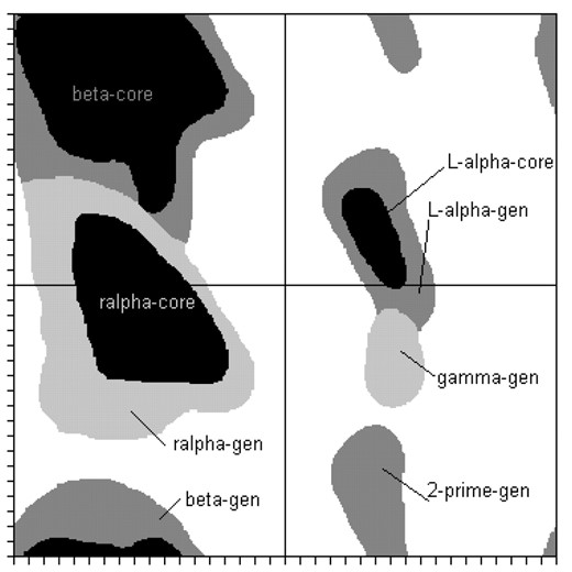
Dihedral regions estimated from (Lovell, 2003). The region interfaces of the generously allowed regions were defined manually by us and are partially overlapping.
Table 1 shows the distribution of the different dihedral angle regions for our dataset. Over 93% are located in the generously allowed alpha and beta regions. Our prediction algorithm belongs to the class of SVM, i.e. a supervised machine-learning algorithm that requires positive and negative examples for training. For a comprehensive introduction to SVMs see (Schoelkopf and Smola, 2002). The C-SVM algorithm implementation of the LIBSVM-library (Author Webpage) with a radial basis function (RBF) kernel is used throughout this study. Input data for training are vectors comprised of a class label and several numerical input values (features). The resulting model is an abstract specification of the hyperplane that separates two classes with the largest margin. This model is then used to classify previously unseen examples. In order to allow the algorithm to harness homology information, we have encoded each amino acid residue of the local sequence neighborhood by a profile vector of amino acid propensities obtained from the position specific scoring matrices of a PSI-BLAST run (Altschul et al., 1997). We use a sliding window of length 15 to define the local sequence environment of a residue. Accordingly, the feature vectors to encode the sequence information are of length 15 × 20 = 300 (Fig. 2).
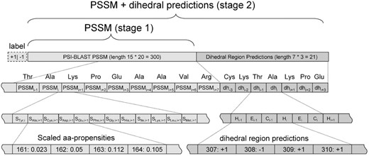
Encoding of vectors for SVM training.
Distribution of dihedral regions where: core = allowed region (union contains 99% of all data according to [Lovell03]), gen = generously allowed region (union contains 99.9% of all data according to [Lovell03])
| Dihedral region (abbrev.) | # of samples |
|---|---|
| Right handed helix, core | 210 840 |
| Right handed helix, gen | 215 391 |
| Beta sheet, core | 174 534 |
| Beta sheet, gen | 182 435 |
| Left handed helix, core | 11 406 |
| Left handed helix, gen | 17 904 |
| II'-region, gen | 2677 |
| Gamma turn, gen | 355 |
| In none of these regions | 7770 |
| In none of this regions, not Glycine | 1003 |
| Total number of residues | 424 609 |
For a second set of classifiers, we also use the predicted class labels obtained from prediction runs using the first SVM-models. We employ a sequence window of length seven and three separate predictions: helix (alpha generously allowed region), extended (beta generously allowed region) and outlier (all others). This gives 21 features, which increase the total length of the vectors for the second set of SVM-models to 321. A sketch of the encoding scheme for both types of classifiers is plotted in Figure 2.
Predictions start by performing a PSI-BLAST run for the target sequence, deriving vectors from the resulting PSSM and obtaining class labels using the first set of SVM-models (step 1). The output of the second step is again a set of three independent predictions for the membership of a residue in the alpha, beta or outlier class, respectively. We find that repeating the second step using the updated dihedral neighborhood information from the previous prediction round leads to further improvement (step 3). In particular, residues showing ambiguous predictions become less frequent. As convergence of this iterative step is not guaranteed, we limit the number of additional rounds to nine. Due to the low number of ambiguous predictions, our use of discrete class labels +1 and −1 (instead of real-valued class probabilities) and a narrow sequence window of only 7 residues for the dihedral neighborhood, we always observe convergence after two to three additional rounds. Remaining ambiguities are resolved by assigning the class label of the nearest non-ambiguous residue (step 4).
Definition of prediction categories for calculation of MCC, specificity and sensitivity
| Prediction | Observation | |
|---|---|---|
| +1 | −1 | |
| +1 | TP (true positive) | FP (false positive) |
| −1 | FN (false negative) | TN (true negative) |
| Prediction | Observation | |
|---|---|---|
| +1 | −1 | |
| +1 | TP (true positive) | FP (false positive) |
| −1 | FN (false negative) | TN (true negative) |
3 RESULTS
3.1 SVM classifier performance
We have initially trained individual classifiers for each dihedral angle region. However, due to the low number of available examples for left handed helices, gamma turns and II′ turns, classifiers for predicting these secondary structure classes show only low correlation on the test set (data not shown). We therefore use here only the information on alpha and beta helices as targets and only train classifiers for two generously allowed regions: right-handed alpha helix and beta strand (denoted ralpha-gen and beta-gen in Fig. 1). A third classifier is trained on residues outside of this both regions. In a first step, we utilize only sequence profile information from PSI-BLAST. For computational reasons we restrict the training set to 20 000 residues from 499 proteins. Our prediction algorithm is then evaluated on an independent test set of 18 872 residues from 97 proteins. Results are shown in Table 3. Already the profile-only SVM classifiers show a prediction performance of ∼80%, in the range of one of the best secondary structure prediction programs, PSIPRED (Jones, 1999). However, note that the models show a marked tendency to over-predict extended residues and to under-predict residues in helical state.
Performance of SVM PSSM-only classifiers
| Region | TP | TN | FP | FN | Acc % | MCC |
|---|---|---|---|---|---|---|
| Alpha H | 7564 | 7924 | 1271 | 2113 | 82.1 | 0.645 |
| Beta E | 6793 | 8631 | 2198 | 1250 | 81.7 | 0.635 |
| Outlier O | 906 | 16 705 | 920 | 341 | 93.3 | 0.567 |
| Region | TP | TN | FP | FN | Acc % | MCC |
|---|---|---|---|---|---|---|
| Alpha H | 7564 | 7924 | 1271 | 2113 | 82.1 | 0.645 |
| Beta E | 6793 | 8631 | 2198 | 1250 | 81.7 | 0.635 |
| Outlier O | 906 | 16 705 | 920 | 341 | 93.3 | 0.567 |
In a second iteration, we improve on these results by adding dihedral neighborhood information obtained from prediction runs using the first classifiers to the training set features. As dihedral neighborhood information, we use the class labels of the first classifiers in a sequence window of length 7 (Fig. 2). Results presented in Table 4 are for the same independent test set of 18 872 residues. As expected, the results in this iteration show a moderate improvement over the predictions from the profile-only classifiers, validating the prediction approach described. The bias towards over-prediction of extended state remains, although less pronounced.
Performance of SVM PSSM + dihedral classifiers
| Region | TP | TN | FP | FN | Acc % | MCC |
|---|---|---|---|---|---|---|
| Alpha H | 7780 | 7971 | 1224 | 1897 | 83.5 | 0.671 |
| Beta E | 6825 | 8861 | 1968 | 1218 | 83.1 | 0.661 |
| Outlier O | 905 | 16 724 | 901 | 342 | 93.4 | 0.570 |
| Region | TP | TN | FP | FN | Acc % | MCC |
|---|---|---|---|---|---|---|
| Alpha H | 7780 | 7971 | 1224 | 1897 | 83.5 | 0.671 |
| Beta E | 6825 | 8861 | 1968 | 1218 | 83.1 | 0.661 |
| Outlier O | 905 | 16 724 | 901 | 342 | 93.4 | 0.570 |
3.2 Comparison to secondary structure prediction programs
Although we are not aware of any programs which yield predictions of a residues dihedral state, some secondary structure prediction programs give probabilities for the secondary structure state of individual residues. Hence, we use this type of output from the GOR-IV and PSIPRED programs as an approximate measure for the dihedral region prediction. We have used the prediction scores without regard of the coil probability, as this purely macroscopic category does not imply any dihedral preference. To estimate the improvement by including information on the 3D environment of similar sequences, we compared our data with PSIPRED predictions obtained in single mode as well as to PSIPRED predictions that use position specific profiles from PSI-BLAST (Table 5).
Prediction test for individual residues (n ≈ 17500)
| DHPRED step 1,2 | PSIPRED profile | PSIPRED single | GOR-IV | ||
|---|---|---|---|---|---|
| Alpha | Sens % | 77 | 86 (64) | 79 (51) | 72 (50) |
| Spec % | 90 | 73 (96) | 60 (85) | 64 (83) | |
| MCC | 0.67 | 0.60 (0.62) | 0.40 (0.38) | 0.35 (0.35) | |
| Beta | Sens % | 80 | 73 (42) | 60 (32) | 64 (34) |
| Spec % | 86 | 86 (96) | 79 (91) | 72 (87) | |
| MCC | 0.66 | 0.60 (0.47) | 0.40 (0.28) | 0.35 (0.25) |
Sensitivity, specificity in % and Matthew's correlation coefficient (mcc). Figures in brackets denote predictions obtained including coil predictions.
Although trained on a smaller database than GOR-IV or PSIPRED, the first two steps of our procedure give the same amount of information on local secondary structure as current secondary structure programs. Our method gives a MCC higher even than PSIPRED. This suggests that PSIPREDs unrivaled ability to detect SSEs comes at the price of a lower ability to detect less uniform local ordering. The low correlation coefficients for predictions including coil underlines that a lot of information about the dihedral state at residue level can be recovered just by ignoring coil prediction probabilities. Note the pronounced improvement in the MCC of ∼0.2 when PSIPRED uses PSI-BLAST profiles. Our own experiments with SVM-based methods, with and without profile information, show a similar gain (data not shown).
3.3 Detailed analysis of CASP6 examples
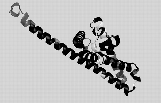
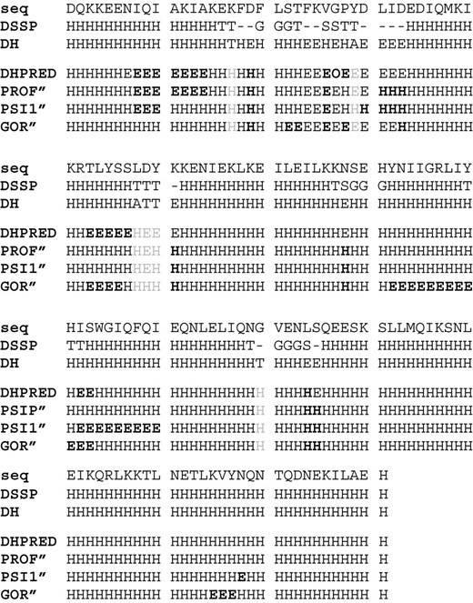
The gold standard for each prediction method is its application to situations where no structure is known for any protein with similar sequence. Consequently, we have tested the performance of our approach for three targets, among them two from the new-fold category of the CASP6. The first test case, Target 242 (PDB-code: 2blk, chain A), shown in Figure 3, is a new-fold and contains long stretches where according to DSSP there are no SSE. DHPRED correctly assigns 72 of the 88 core residues (81.8%) including all three ‘outliers’, while PSIPRED predicted 70 (79.6%). GOR-IV, in contrast, predicts less than half of the residues correctly, emphasizing that, even for new-folds, implicit information on the 3D environment can be obtained using sequence profiles. The correctly predicted regions are colored in black in Figure 3, while white denotes false predictions and gray the termini, and outlier residues, which have not been evaluated in the comparison. A more detailed listing of our results for this protein and a comparison with competing techniques, can be found in Figure 4. The false predictions for target 242 are mainly located in four clusters. The C-terminal part of the first alpha helix is not recognized, an error, which is, even more pronounced in the PSIPRED prediction. Before the second helix, an alternating pattern is missed and two patterns where DSSP reports turns are not correctly predicted. The correlation of mispredictions between PSIPRED and DHPRED makes it likely that in these regions either rare H-bonding patterns occur or the normal local structure is strongly influenced by non-local interactions.
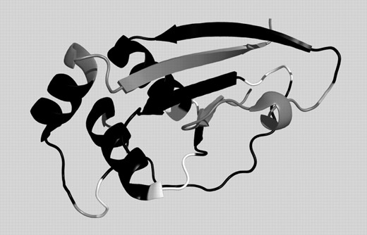
Prediction for CASP6 target 242 (2blkA). Black: correct prediction, white: wrong prediction, gray: not evaluated (chain ends and outliers).
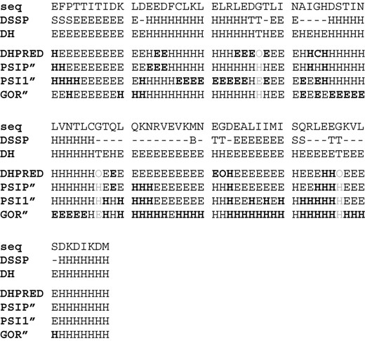
True dihedral state and predictions for CASP6 target 242 (2blkA) with different algorithms. Normal face: correct, bold: wrong, gray: not evaluated. seq = amino acid sequence in one-letter-code, DSSP = secondary structure annotation by DSSP, DH = dihedral region according to the Lovell definitions: E = within beta-gen (extended), H = within ralpha-gen, O = outside of both regions (turn), DHPRED: dihedral region predicted by our SVM approach, GOR′: predicted preference by GOR-IV when ignoring coil prediction, PSI1′: same for PSIPRED without using profile information, PSIP′: same for PSIPRED using profile information.
Our second test case is the new-fold target 238 (PDB-code: 1w33, complement protein), which has an all-alpha structure and is shown in Figure 5. In spite of the tendency of DHPRED to under-predict residues in helical state, it assigns 86.9% of the 145 core residues to the correct class. Here PSIPRED, which favors helix predictions, achieves slightly better results (89.0%). The detailed analysis of Figure 6 demonstrates that false predictions by the SVM method cluster at the C-terminal half of the first and second helix. The first cluster of mispredictions is shared with PSIPRED. A scattered cluster of mispredictions is also located at the complex loop structure between the first and second helix. The first cluster of mispredictions contains the subpattern Ile-Gln-Ile (IQI), which is found more frequently in beta sheets than in alpha helices. The same is true for second missed pattern, Lys-Tyr-Ser-Ser (LYSS). Due to our small number of training residues, we may have missed the less frequent sequence profiles, which belong to helical conformations of this pattern.
Prediction for CASP6 target 238 (1w33A). Black: correct prediction, white: wrong prediction, gray: not evaluated (chain ends and outliers).
True dihedral state and predictions for CASP6 target 238 (1w33A) with different algorithms. Normal font: correct prediction, bold font: wrong prediction, gray: not evaluated (ambiguous or outliers). (Fig. 4. for detailed legend).
Although, not a new-fold, the third test case, Target 273 (PDB-code: 1wdj), was chosen for its complex alpha-beta topology that includes a beta barrel at the C-terminus. The molecule is displayed in Figure 7. The prediction accuracy of DHPRED (82.4%) is even higher than that of PSIPRED. Although, the large number of different loop structures connecting the SSE is the main problems for the DHPRED predictor, it assigns 33 of 51 (64.7%) correctly, while the residue dihedral state of PSIPRED is only correct in 49.0% of the cases (Fig. 8 and Table 7).
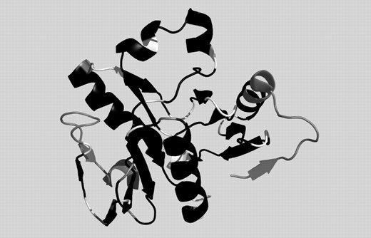
Prediction for CASP6 target 273 (1wdjA). Black: correct prediction, white: wrong prediction, gray: not evaluated (chain ends and outliers).
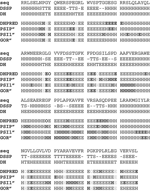
True dihedral state and predictions for CASP6 target 273 (1wdjA) with different algorithms. Normal font: correct prediction, bold font: wrong prediction, gray: not evaluated (ambiguous or outliers). (Fig. 4. for detailed legend).
Tables 6 and 7 summarize the results for the three targets. Note that in all three cases false predictions tend to cluster and that all methods show strong correlations on the residues for which they predict the wrong class. While this is not surprising for residues within ‘coil’ regions with their irregular H-bond pattern, we find such ‘difficult residues’ also in helices that have neither strong kinks nor bends. The observed correlation of false predictions between three independent methods implies that in these particular regions the local structures strongly deviate from the average structures observed for similar sequences. We conjecture that in these cases the local secondary structure is more strongly determined by the non-local environment of the surrounding protein than it is on average. This is a principal limitation of all techniques that use only local sequence information.
Performance comparison on three targets from CASP6
| CASP target (pdb) | T0238 (2blkA) | T0242 (1w33A) | T0273 (1wdjA) |
|---|---|---|---|
| Res | 85–235 | 17–104 | 17–172 |
| # Res | 151 | 88 | 156 |
| # Res eval | 145 | 85 | 148 |
| % Correctly assigned | |||
| GOR-IV″ | 80.0 | 48.2 | 75.7 |
| PSIPRED single″ | 84.1 | 62.4 | 68.9 |
| PSIPRED profile″ | 89.0 | 82.4 | 80.4 |
| SVM-DH | 69.6 | 60.0 | 79.1 |
| DHPRED step 1 | 75.2 | 74.1 | 75.0 |
| DHPRED step 1,2 | 85.5 | 77.7 | 80.4 |
| DHPRED step 1,2,3 | 86.9 | 78.8 | 81.1 |
| DHPRED step 1,2,3,4 | 86.9 | 81.2 | 82.4 |
Performance comparison in regions without SSEs
| CASP target (pdb) | T0238 (2blkA) | T0242 (1w33A) | T0273 (1wdjA) |
|---|---|---|---|
| # Res eval | 145 | 85 | 148 |
| # Res w/o SSE | 22 | 35 | 51 |
| % Correctly assigned | |||
| PSIPRED profile″ | 59.1 | 65.7 | 49.0 |
| DHPRED step 1,2,3,4 | 77.3 | 65.7 | 64.7 |
| CASP target (pdb) | T0238 (2blkA) | T0242 (1w33A) | T0273 (1wdjA) |
|---|---|---|---|
| # Res eval | 145 | 85 | 148 |
| # Res w/o SSE | 22 | 35 | 51 |
| % Correctly assigned | |||
| PSIPRED profile″ | 59.1 | 65.7 | 49.0 |
| DHPRED step 1,2,3,4 | 77.3 | 65.7 | 64.7 |
4 CONCLUSION AND OUTLOOK
We have developed a multi-step SVM-procedure DHPRED for predicting the dihedral class of individual residues. The advantage of such an approach over conventional secondary structure prediction methods is twofold. First, some of the difficulties arising from the inherent complexity of secondary structure definitions are avoided and second, it leads to additional information in ‘coil’ regions. Our approach is based solely on sequence profiles. However, each step generates additional information on the dihedral neighborhood that is used in the following step to improve the prediction performance. The method compares favorably to non-profile methods and is on par with PSIPRED regarding the overall prediction quality.
While PSIPRED excels especially on proteins with high helix content, DHPRED shows much higher prediction accuracy in regions between SSE. For computational reasons, we have used a rather small training set (20 000 residues from 499 proteins). We expect that larger training sets and rigorous parameter optimization will improve the prediction results considerably. In the future, we plan to use parallelized implementations of SVM algorithms that will allow for the weighting of features. We will also try to address some of the shortcomings of DHPRED e.g. employing special training sets for Glycine and Proline, which have dihedral preferences that deviate considerably from those of the other amino acid residues. Starting from microscopic predictions, as in DHPRED, we intend to target the prediction of macroscopic secondary structure in a bottom-up approach.
This work is supported in part by a research grant (GM62838) of the National Institutes of Health. The computations were performed on Computers at the John v. Neumann Institute for Computing in Jülich, Germany.
Conflict of Interest: none declared.
REFERENCES
Author notes
Associate Editor: Anna Tramontano

