Late Mitochondrial Origin Is an Artifact

Abstract

In a recent report, Pittis and Gabaldón (2016) claimed to have presented evidence that the mitochondrion came late in the process of eukaryotic origin, following an earlier phase of evolution in which the eukaryotic host lineage acquired genes from bacteria. Here, we subject their report to critical inspection. For 1,078 phylogenetic trees containing prokaryotic and eukaryotic homologues, Pittis and Gabaldón (2016) calculated the length of the branch subtending the eukaryotic clade (raw stem length, rsl) relative to the median root-to-tip length of lineages within the eukaryotic clade (eukaryotic branch length, ebl_med), a value they call stem length (sl). From variation in sl, they infer early (large sl) and late (small sl) gene acquisitions in eukaryotes, using sl as a measure for age. They feed values of sl into the expectation maximization (EM) algorithm to sort the data into five Gaussian components spanning small to large sl values. One of the five components contained 14 very large values, which they exclude from further analysis. The remaining 1,064 values of sl, which EM had sorted into four components, are subjected to various analyses, results of which they interpret as evidence that some genes entered the eukaryote lineage early (component 4), some later (component 3), some later yet (component 2) and the largest portion finally entering with the mitochondrion (component 1).

The first question is: Are these four components real? No. They are an artifact produced by the overfitting of a complex (14 parameters) Gaussian mixture model, when a much simpler (2 parameters) log-normal model better explains the data. The sl data of Pittis and Gabaldón, which we show in figure1a for inspection, are not multiple Gaussian distributed with five components, they are log-normally distributed, as borne out by both the Akaike and the Bayesian information criteria (fig. 1b). This is a fatal flaw of Pittis and Gabaldón (2016). Their four (five-exclude-one) Gaussian groups, or components, are a methodological artifact. All analyses, tests and far-reaching inferences about eukaryote origin based upon the four Gaussian mixture components (Pittis and Gabaldón 2016) of sl are not just erroneous, they are meaningless, because the data are not normally distributed, with five components or otherwise.

Fig. 1.—

Open in new tabDownload slide

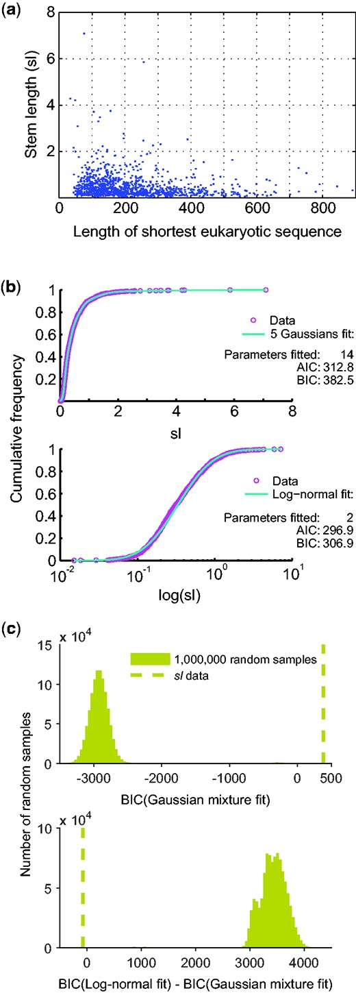
Distribution of 1,078 stem length (sl) values. (a) sl as a function of sample size (eukaryotic sequence length). (b) Fit of the sl values to a five Gaussian mixture model (top), and to a log-normal model (bottom). AIC: Akaike information criterion, BIC: Bayesian information criterion. Note that the log-normal distribution is strongly preferred. (c) 1,000,000 random samples from a 5-Gaussian mixture model were generated with the parameters estimated from the observed stem length (sl) data obtained by Pittis and Gabaldón (2016). Top: BIC for the fitting of each of the 1,000,000 random samples (bars) and the observed sl data (dashed line) to a Gaussian mixture model from 1 to 7 components. Bottom: Difference between BIC for the fitting to a log-normal distribution and to a Gaussian mixture model from 1 to 7 components for each of the 1,000,000 random samples (bars) and for the observed sl data (dashed line). BIC, Bayesian information criterion.

How do they obtain a five-component mixture model for sl? They incorrectly treat the sl values as normally distributed. The sl values are ratios, hence strictly positive, with mean 0.48, standard deviation (SD) 0.54, and skewness 4.7. Because negative values are within one SD from the mean, and because the distribution is not symmetrical, the sl values cannot possibly be normally distributed. For data with such features, a logarithmic transformation is to be examined (Zar 2010). The transformed sl values do fit a Gaussian, that is, the sl values should be modeled by a log-normal distribution. Elementary statistical procedures were neglected, and since one Gaussian did not fit the data, more Gaussians were needlessly presumed (Pittis and Gabaldón 2016). This is a textbook case of overfitting, where the addition of new parameters increases the apparent fit (fig. 1b), even when the underlying model is inappropriate. The EM program reproducibly generates 3–7 Gaussian components from randomly generated, perfectly log-normal data (see Materials and Methods section) of the sample size, mean, and variance reported in Pittis and Gabaldón (2016).

To be critical, however, we also have to check another possibility: Could it be that data drawn from a Gaussian mixture somehow artifactually produce a better fit to a log-normal distribution? To check this, we generated one million random samples from the 5-Gaussian mixture with the parameters estimated from the observed sl data, and fitted the distributions to both a log-normal model and a Gaussian mixture (allowing from 1 to 7 components). The BIC of the observed data is inferior to every one of the one million Gaussian mixture random samples generated (fig. 1c), and the likelihood of the empirical data is smaller than that of the average random sample by a factor of 10⁷¹⁴. Moreover, not in a single case did we observe a better fit of Gaussian mixture generated data to the log-normal model (fig. 1c). This shows that for data that (i) is drawn from a 5-Gaussian mixture and (ii) that has parameters corresponding to the observed sl data, the chance to get a better fit to a log-normal distribution is less than one in a million (P value < 10⁻⁶).

The partitioning of Pittis and Gabaldón’s (2016),sl data into four (five exclude one) components, the central pillar of their paper, is thus fatally flawed. But so is the use of sl values to draw inferences about evolutionary time. Because different gene families evolve at different rates, the raw rsl distances are normalized by ebl_med, which is claimed to reflect, for each gene family, a characteristic eukaryotic evolutionary rate that was constant across all lineages and times during eukaryotic evolution: a root-to-tip molecular clock for each tree. A clock assumption might hold for some gene families (Bromham and Penny 2003), but it does not hold for the majority of the 1,078 families reported (Pittis and Gabaldón 2016). The full set of ebl values for each gene family reveals extreme variation, with a mean per-family coefficient of variation of 27%, and a median longest-to-shortest within family ebl ratio of 2.2. Across their 1,078 trees (Pittis and Gabaldón 2016), the largest value of ebl exceeds that of the shortest by >2-fold—on average. Clearly, the molecular clock assumption is not met, and ebl_med is neither characteristic nor constant (fig. 2).

Fig. 2.—

Open in new tabDownload slide

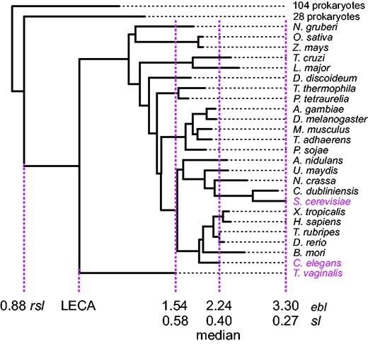
Phylogenetic tree and sl derivation for COG4178_01, an ABC transporter present in 25 eukaryotic taxa. Which eukaryotic branch length (ebl) should be used to calibrate the raw stem length (rsl)? The minimal, median, and maximal lineages are highlighted in magenta. Perchance it is a moot question, as in the absence of a LECA-to-present molecular clock, none of the resulting sl values convey meaningful information. The ratio of longest to shortest ebl is 2.15, a value representative of the data set as 579 other trees have larger ratios.

Dividing rsl by ebl_med to produce sl is then bound to yield arbitrary values, which it does, and the interpretation of these values as measures of divergence times culminates in absurd results. How so?

Eukaryotes are at least 1.6–1.8 billion years (Ga) in age (Parfrey et al. 2011). If one uses sl as a measure for the age of genes that eukaryotes acquired from prokaryotes (Pittis and Gabaldón 2016), variation in sl implies continuous eukaryotic gene acquisition from prokaryotes starting >4.5 Ga ago, before Earth’s formation. That seems unlikely. Where is the error? Examining values of sl for groups within eukaryotic phylogeny are instructive. Crucially, all well-sampled eukaryotic groups show variation and distribution of sl virtually identical to that of eukaryotes as a whole (fig. 3). The log-normal distribution again fits the data best, yet it is all-too-easy to use EM to overfit a Gaussian mixture model with multiple components. For example, the value of sl for metazoans, as defined (Pittis and Gabaldón 2016), indicates the age of the metazoan stem lineage after divergence from other eukaryotes relative to the age of the metazoan crown. Taking the crown age of metazoans (Parfrey et al. 2011, Benton and Donoghue 2007) as ∼1 Ga, and using sl as a proxy for age (Pittis and Gabaldón 2016), the metazoan stem lineage, with sl ranging from ∼0.1 to ∼3, diverged continuously from its eukaryotic sister group during the time ∼0.1 to ∼3 Ga before the first metazoan arose ∼1 Ga ago, which cannot be true. We have a far less radical alternative explanation: sl is not an indicator of gene age differences within or between trees at all, rather sl vividly documents abundant branch length variation within and among Pittis and Gabaldón’s trees, stemming from rate variation within and among lineages across trees, which is well-known to exist, which is expected (Bromham and Penny 2003, Parfrey et al. 2011, Williams et al. 2013, Ho et al. 2016, Phillips 2016), and which can be readily grasped by looking at their actual trees (fig. 2).

Fig. 3.—

Open in new tabDownload slide

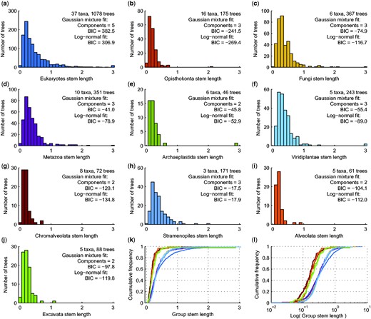
Stem length (sl) distributions among eukaryotes and the fit to Gaussian mixture and log-normal models. (a–j) Histograms of group specific sl for the largest clade containing only group members with taxa from at least two taxonomic subgroups. Values in panel (a) are from Pittis and Gabaldón (2016), values in panels (b–j) were calculated from the trees in Pittis and Gabaldón (2016). In panels (a–j), the rightmost bin contains all values ≥3; AIC: Akaike information criterion, BIC: Bayesian information criterion. (k–l) Empirical cumulative distribution functions for the sl values in panels (a–j), in sl scale (k) and log(sl) scale (l). Colors match the colors used in (a–j).

What that means is this: Either Pittis and Gabaldón (2016) assume that (i) the relative substitution rate in the stem and eukaryotic lineages is the same for every protein or, alternatively, they assume that (ii) the relative substitution rates for any two chosen proteins from the 1,078 they examined remained the same before and after LECA (or they assume both (i) and (ii).

Are such assumptions tenable? Observation and theory alike suggest that the equalities (4) are not likely in general. The reasons are manifold. First, what is $R e$? Pittis and Gabaldón use the median $K e$ (ebl_med) as a proxy, but in different gene families the median is obtained in different organisms as dissimilar as Trichomonas vaginalis, Homo sapiens and Oryza sativa in their sample. With such a range of mutation rates, generation times, population sizes and sexual recombination or its absence, the variable substitution rates seen in the several lineages of each gene family are anything but surprising. Conceivably, this pitfall could have been avoided by using a single reference eukaryotic lineage instead of the arbitrary lineages presenting the median.

Yet equalities (4) are even more suspect when considering the selective regimes operating in different lineages and on different genes. Of particular interest here is the proto-eukaryotic, or stem, lineage. What can we expect of the substitution rates in this lineage: Were they similar to those of the archaeal host, to those of the proteobacterial symbiont, or to those of any of the eukaryotic descendant lineages? Probably all of the above, depending upon the gene and the lineage, with the additional complications of changing selective constraints accompanying one of the major evolutionary transitions in the history of life. It is to be expected that during eukaryogenesis different genes reacted differently in terms of functional constraints and substitution rates, especially for genes that were acquired from endosymbionts (Martin and Herrmann 1998). Modern investigations that strive to infer the relative timing of events even as recent as placental mammal radiation (<0.1 Ga) from molecular sequence data underscore the need to allow the substitution rate to vary across the tree in order to account for the data (Phillips 2016). For more ancient events, the same holds true. The implicit assumption that evolutionary rates before and after LECA for a given protein family are correlated (⁠ $R s i R e i = R s j R e j )$⁠, or that relative substitution rates of two different protein families remained constant throughout time (⁠ $R s i R s j = R e i R e j$⁠), is the basis of the molecular clock assumption that Pittis and Gabaldón (2016) embrace without explicitly saying so. That assumption was neither tested in their paper, nor is it likely to hold. As Ho et al. (2016) put it in their recent review: “Any particular molecular clock is unlikely to be reliable across a broad range of timeframes.” The several billion year timeframe considered in Pittis and Gabaldón (2016) would qualify as broad.

In addition, their 1,078 trees (Pittis and Gabaldón 2016) are not independent samples of the data. Starting from 883 EggNOG clusters, 722 clusters were used once, 130 twice, 28 thrice, and 3 clusters in four trees. Trees showing eukaryote polyphyly were split and scored as multiple eukaryote monophyly (Pittis and Gabaldón 2016). Their 1,078 trees contain 403,451 sequences: 238,080 occur once, 5 occur in seven trees, 3 in six, 53 in five, 2318 in four, 14,645 in three, and 55,923 sequences occur in two different trees. Moreover, their statistical analysis of α-proteobacterial versus bacterial but non-α-proteobacterial gene classes hinges upon rare and/or anomalous data: if alignments containing very short, highly gapped or otherwise tenuous attributes are removed, or if analyses are properly restricted to their 722 independent samples, their borderline significance values suggesting two classes disappear completely (fig. 4).

Fig. 4.—

Open in new tabDownload slide

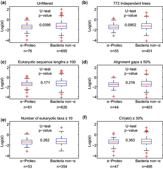
Comparison of stem length (sl) values in classification of the prokaryotic sister clade as α-proteobacterial or bacterial but non-α-proteobacterial. (a) Unfiltered: full data set analyzed in Pittis and Gabaldón (2016). (b–f) Data sets obtained by exclusion of questionable, low-quality, or nonindependent sample points. n: number of observations, U-test: Mann–Whitney U test; CV, coefficient of variation.

Unnoted by Pittis and Gabaldón (2016), an earlier study analyzed more than three times as many independent trees (Ku, Nelson-Sathi, Roettger, Sousa, et al. 2015). In that study, all sequences were unique, eukaryote nonmonophyly was scored as such, not as multiple observations of eukaryote monophyly (Pittis and Gabaldón 2016), and the data uncovered neither evidence for a late mitochondrion, nor for a late plastid (Ku, Nelson-Sathi, Roettger, Sousa, et al. 2015).

Another major flaw of Pittis and Gabaldón (2016) is their complete disregard of LGT among prokaryotes (Ku, Nelson-Sathi, Roettger, Garg, et al. 2015; Ku, Nelson-Sathi, Roettger, Sousa, et al. 2015), which, along with differential loss, strongly influences the dynamic gene contents of prokaryotes (Gogarten and Townsend 2005; Koonin and Wolf 2008; Ochman et al. 2000). In the view of Pittis and Gabaldón (2016), only genes whose sister groups consist of present-day α-proteobacteria in their data set—a tiny sample of bacterial gene diversity (Wu et al. 2009)—can be regarded as being of “α-proteobacterial ancestry,” and hence, in their reasoning, as being of mitochondrial origin. Their assertion that LGT “cannot explain the observed signal from non-α-proteobacterial bacteria” is based on their Extended Data figure 6 in Pittis and Gabaldón (2016), with two scenarios (upper row in panel b; hereafter X and Y) where LGT among bacteria and gene loss (or incomplete sampling) would result in eukaryotic genes of mitochondrial origin having non-α groups in trees. If a tree corresponds to scenario X, rsl/sl should be no different from the situation where the gene still has α-proteobacteria in the sister group; if it is Y, rsl/sl should be larger. To test these scenarios (Pittis and Gabaldón 2016, Supporting Information Section 4), the authors compared sl of trees with different sister groups. They found that sl of the trees with non-α in the sister group is larger than, rather than the same as, those with α-proteobacteria (Pittis and Gabaldón 2016, fig. 2), from which they concluded that scenario X cannot explain the observation of nonα sister groups. Then they found that sl of the trees reinferred after all α-proteobacteria were removed (simulating gene loss in α-proteobacteria) is even larger than that of the original trees with nonα sisters (Pittis and Gabaldón 2016, Extended Data fig. 6c), so they concluded that the larger sl (Pittis and Gabaldón 2016, fig. 2) cannot be explained by scenario Y and that both scenarios can be ignored. The fallacy in their reasoning is the assumption that genes with nonα sisters correspond either all to X or all to Y. It is far more probable that some genes correspond to X whereas the others to Y. This is why the original non-α sl (mixture of X and Y) is larger than the original α sl due to the existence of some Y trees, but smaller than the newly generated sl (with additional Y trees generated by simulated removal of α-proteobacteria). Lateral transfer among prokaryotes and gene loss in prokaryotes are very important issues when it comes to inferring the origin of eukaryotic genes in the context of endosymbiosis (Martin 1999; Ku, Nelson-Sathi, Roettger, Garg, et al. 2015). But LGT among prokaryotes and genes loss (Ku, Nelson-Sathi, Roettger, Garg, et al. 2015; Ku, Nelson-Sathi, Roettger, Sousa, et al. 2015) were disregarded by Pittis and Gabaldón (2016). The perhaps simplest interpretation of Pittis and Gabaldón’s observations concerning branch length variation is that for genes of mitochondrial origin, the less the eukaryotic protein has to do with its original function in the free-living mitochondrial ancestor, the longer the branch becomes that links it to its prokaryotic homologues.

In summary, sl-based conclusions about eukaryote evolution (Pittis and Gabaldón 2016) are unfounded, resting upon fatal flaws in (i) overfitting of the wrong distribution model, (ii) analyses of non-independent data, and (iii) implicit, untested, and untrue molecular clock assumptions.

Materials and Methods

All analyses were based on alignments and phylogenetic trees kindly provided by T. Gabaldón. No realignments or reinference of trees was carried out. Values of rsl and ebl were extracted from the trees, values of sl were recalculated, reproducing the values reported in Pittis and Gabaldón (2016). For calculating sl within eukaryotic groups, trees were searched for the largest clade containing only group members with taxa from at least two different taxonomic subgroups. All statistical analyses were performed using the MatLab statistics toolbox.

Author Contributions

W.F.M., M.R., C.K., S.G.G., S.N.-S., and G.L. designed experiments, analyzed data, and prepared this manuscript; M.R., C.K., S.N.-S., and G.L. performed computational analysis.

Acknowledgments

We thank the Zentrum für Informations- und Medientechnologie (ZIM) of the Heinrich-Heine University for computational support and the European Research Council for funding (ERC AdG 666053 to W.F.M.). G.L. was supported by the European Research Council (Grant No. 281357 to Tal Dagan). The authors declare no competing financial interests.

Literature Cited

Author notes