


Abstract
We present a statistical analysis of the millimetre-wavelength properties of 1.4 GHz-selected sources and a detection of the Sunyaev–Zel'dovich (SZ) effect associated with the haloes that host them. We stack data at 148, 218 and 277 GHz from the Atacama Cosmology Telescope at the positions of a large sample of radio AGN selected at 1.4 GHz. The thermal SZ effect associated with the haloes that host the AGN is detected at the 5σ level through its spectral signature, representing a statistical detection of the SZ effect in some of the lowest mass haloes (average M200 ≈ 1013 M|$_{{\odot }}\,h_{70}^{-1}$|) studied to date. The relation between the SZ effect and mass (based on weak lensing measurements of radio galaxies) is consistent with that measured by Planck for local bright galaxies. In the context of galaxy evolution models, this study confirms that galaxies with radio AGN also typically support hot gaseous haloes. Adding Herschel observations allows us to show that the SZ signal is not significantly contaminated by dust emission. Finally, we analyse the contribution of radio sources to the angular power spectrum of the cosmic microwave background.
INTRODUCTION
In the standard cosmological structure formation scenario, astrophysical structures (galaxies, galaxy groups and clusters) form when gas condenses at the centres of hierarchically merging dark matter haloes (White & Rees 1978). The accretion is characterized according to two modes: radiatively efficient and radiatively inefficient (Binney 1977; Rees & Ostriker 1977; Silk 1977). In the radiatively efficient rapid-cooling mode, the gas is shock heated within the virial radius of the dark matter halo, and as it cools it accretes on to the galactic disc, contributing to star formation. In the hydrostatic (hot) mode, the gas is shock heated before reaching the virial radius, and a hydrostatically supported gaseous halo forms. This gaseous halo radiates in X-ray wavelengths, and as it radiatively cools, it has the capacity to form stars. However, large cooling flows accompanied by prodigious star formation are not observed: the predominant stellar populations at the centres of the most massive haloes are old and red, and X-ray measurements indicate a lack of cool gas compared to the level expected from the cooling (e.g. Oegerle et al. 2001; Peterson et al. 2003). One mechanism invoked to explain this problem is feedback from active galactic nuclei (AGN). Radiatively inefficient accretion can power a ‘radio mode’ AGN, where the gas that accretes on to the AGN ultimately comes from the hot gaseous halo. Because the radio AGN can deposit energy back into this gaseous halo, a feedback mechanism can form that regulates the gas in a way that prevents both catastrophic cooling and excessive star formation. Evidence for the existence of such feedback comes from a number of different observations (for a review, see McNamara & Nulsen 2007). Cavities or bubbles are observed in the X-ray haloes of nearby galaxy clusters that are filled with radio emission (e.g. Fabian et al. 2000; McNamara et al. 2000). Galaxy evolution models that include this feedback mechanism can successfully reproduce observed galaxy luminosity functions (e.g. Bower et al. 2006; Croton et al. 2006; Sijacki et al. 2007). The correlation of the prevalence of low-luminosity radio AGN with stellar mass, black hole mass, galaxy velocity dispersion and colour also provides support for the presence of radio mode feedback (e.g. Best et al. 2005; Best & Heckman 2012). That radio-loud AGN tend to reside in relatively massive (∼1013 M|$_{{\odot }}\,h_{70}^{-1}$|) dark matter haloes has been confirmed by studies of the clustering of galaxies around radio AGN (Overzier et al. 2003; Magliocchetti et al. 2004) and by stacked weak lensing (Mandelbaum et al. 2009). However, the gaseous content is more challenging to observe, with recent X-ray studies currently restricted to dozens of systems (Ineson et al. 2013).
Sensitive millimetre-wave observations have the potential to reveal the Sunyaev–Zel'dovich (SZ) effect of the hot gas associated with radio AGN. The SZ effect is a spectral distortion in the cosmic microwave background (CMB) that occurs when CMB photons inverse-Compton scatter off of the hot ionized gas associated with dark matter haloes. The thermal SZ effect appears as a temperature decrement below (and increment above) ∼220 GHz, at which frequency there is no distortion (Sunyaev & Zel'dovich 1970). The amplitude is effectively independent of redshift (for a review, see Carlstrom, Holder & Reese 2002). Given the mass of the AGN-hosting dark matter haloes, a simple extrapolation of SZ-mass relations derived from more massive haloes (e.g. Sifón et al. 2013) reveals that the SZ effect in 1.4 GHz selected AGN should offset the non-thermal millimetre emission at 148 GHz by a significant (∼50 per cent) fraction. The Planck Collaboration (2013b) recently reported a detection of the SZ effect of haloes of similar mass that they selected via stellar mass. These observations suggest the feasibility of measuring the SZ effect from the haloes that host radio-loud AGN with existing data sets. If the SZ effect can be separated from the synchrotron source spectral behaviour, we can provide evidence of the existence of hot gas atmospheres in dark matter haloes hosting galaxies with radio-loud AGN.
At flux densities above 1 mJy, counts of 1.4 GHz radio sources are dominated by AGN that span a wide range in redshift, with median redshift ∼1 (Condon 1989). The synchrotron spectral behaviour of radio sources is complex and varies significantly from source to source (e.g. Sadler et al. 2006; Lin et al. 2009; de Zotti et al. 2010; Sajina et al. 2011). Models describing radio source spectral behaviour often characterize sources into two types: flat spectrum (α ∼ 0, where α is defined such that S ∝ ν−α) and steep spectrum (α ∼ 0.8). Optically thin synchrotron emission, usually associated with radio lobes, results in a steep-spectrum source, while optically thick emission, usually associated with compact cores, results in a flattened spectrum source (e.g. de Zotti et al. 2010). Using optical observations and radio data at multiple frequencies, the counts of 1.4 GHz sources have been successfully modelled with radio luminosity functions associated with these two populations (e.g. Condon 1984; Peacock 1985; Danese et al. 1987; de Zotti et al. 2005; Massardi et al. 2010), with the flat-spectrum population emerging as faint sources at z = 1. These radio luminosity functions have been extrapolated, assuming a spectral index, to the millimetre regime where they have been used to predict the source population, especially for use in foreground models of CMB data (CMB; e.g. Toffolatti et al. 1998; de Zotti et al. 2005; Sehgal et al. 2010; Tucci et al. 2011). In addition to the synchrotron emission from the AGN, the AGN host galaxies can contain dusty star-forming regions, as have been previously investigated by e.g. Seymour et al. (2011). With the advent of large-scale millimetre-wave surveys with mJy sensitivities and the availability of infrared (IR) surveys with Herschel,1 we can now directly test the spectral behaviour of 1.4 GHz-selected radio-loud AGN across two decades of frequency.
In addition to the AGN population that dominates at S1.4 > 1 mJy, deep radio surveys at 1.4 GHz (20 cm) (e.g. Condon 1984; Becker, White & Helfand 1995; Condon et al. 1998; Hopkins et al. 1998; Mauch et al. 2003) have revealed an excess number of sources at faint radio flux densities, typically with an upturn in the number counts below ∼1 mJy. The observed excess has been mostly attributed to the emergence of a population of spiral galaxies undergoing significant star formation (e.g. Condon 1992; Hopkins et al. 1998), although with some contribution from low-power AGN (e.g. Seymour et al. 2008). These star-forming galaxies (SFGs) are the predominant population below 0.1 mJy and account for ≳ 20 per cent of the population below S ∼ 1 mJy. The radio emission from SFGs comes from synchrotron radiation associated with supernova remnants. In the far-infrared (FIR), and similarly into the submillimetre regime, SFG emission is predominantly thermal from the absorption and re-emission of starlight by dust grains and is described as a grey body with a spectrum rising with frequency (S ∼ ν3.5; Draine 2003).
In this study, we stack 148, 218 and 277 GHz observations from the Atacama Cosmology Telescope (ACT) corresponding to the locations of 1.4 GHz selected radio sources to determine the average millimetre emission associated with radio sources as a function of 1.4 GHz flux density. We also utilize radio data from surveys conducted by Parkes and the Green Bank Telescope (GBT) and IR data from surveys conducted by Herschel to constrain the median spectral energy distributions (SEDs) of radio sources over the frequency range of 1.4 up to 1200 GHz. We use Faint Images of the Radio Sky at Twenty Centimetres (FIRST) sources matched to National Radio Astronomy Observatory Very Large Array Sky Survey (NVSS) sources through the cross-matched catalogues provided by Best & Heckman (2012) and Kimball & Ivezić (2008). This enables us to benefit from both the 1 arcsec astrometric precision of the FIRST survey, and the ability of the larger (45 arcsec full width at half-maximum, FWHM) NVSS beam to recover more extended radio emission. By modelling the observed flux densities, we estimate the average spectral behaviour of low-frequency sources from 1.4 to 1200 GHz and find a robust detection of the SZ effect in radio-loud AGN haloes, particularly evident at 148 GHz.
This paper is organized as follows. Section 2 describes the data from ACT, the 1.4 GHz radio source samples, the IR data, and additional 5 GHz radio survey data used. Section 3 presents the median SEDs for AGN and for SFGs from a relatively low-redshift radio source sample constructed by Best & Heckman (2012) by matching radio sources with galaxies with spectroscopic measurements from Sloan Digital Sky Survey (SDSS), as well as the results of modelling different components of these SEDs. In Section 4, we extend this analysis to a larger sample of radio sources from Kimball & Ivezić (2008) that extends to higher redshift, albeit a sample that lacks optical counterpart identification, and split the sample into bins of 1.4 GHz flux density. Finally, we discuss and summarize our results and their implications for the SZ effect for the typical radio AGN halo and for the CMB power spectrum in Sections 5 and 6. Unless specified otherwise, we assume a flat Λ cold dark matter cosmology with Ωm = 0.30 and |$\Omega _\Lambda =0.70$|. For the Hubble constant, we adopt the notation H0 = 70 h70 km s−1 Mpc−1, and E(z) describes the evolution of the Hubble parameter and is defined as |$E(z) = \sqrt{\Omega _{\rm M}(1+z)^3 + \Omega _{\Lambda }}$|.
DATA
ACT data
ACT is a 6 m, off-axis Gregorian telescope in the Atacama Desert of Chile at an altitude of 5200 m (Swetz et al. 2011). The location was chosen for the atmospheric transparency at millimetre wavelengths and the ability to observe both northern and southern celestial hemispheres. ACT had four observing seasons between 2007 and 2010 and surveyed both a southern celestial hemisphere region (δ = −53| $_{.}^{\circ}$|5) and an equatorial region. ACT observed simultaneously in three frequency bands centred on 148 GHz (2.0 mm), 218 GHz (1.4 mm) and 277 GHz (1.1 mm) with angular resolutions of 1.4, 1.0 and 0.9 arcmin, respectively. Each band had a dedicated array of 1024 transition edge sensors. This paper uses the 2009–2010 148 GHz, 2009–2010 218 GHz and 2010 277 GHz equatorial observations.
Prior to all other analyses described in this paper, the ACT data were matched filtered (cf. Tegmark & de Oliveira-Costa 1998) with the ACT beam (Hasselfield et al. 2013b, for more details see Section 2.1.1) in order to increase the signal-to-noise ratio of compact sources. The filtering procedure is the same as described in Marsden et al. (2014). Each map for each season was calibrated separately (for uncertainties in overall calibration, see Section 2.1.1) and filtered with the beam appropriate for that season and band. The resulting calibrated, filtered maps were combined into a multiseason map via a weighted average, with the weights set for each pixel by the number of observations. The ACT sensitivity varies throughout the maps according to the depth of coverage. The typical rms noise level is 2.2, 3.3 and 6.5 mJy for 148, 218 and 277 GHz, respectively.
The ACT equatorial region contains detectable levels of Galactic cirrus emission. In order to check whether Galactic contamination affects our results, we applied the dust mask used in the analysis of the angular power spectrum of the ACT data (Das et al. 2014). This mask was generated using data from the Infrared Astronomical Satellite (IRAS) as processed by IRIS (Miville-Deschênes & Lagache 2005). Our results are not significantly affected when we mask the regions with strongest dust emission.
Calibration
The uncertainty on the absolute temperature calibration of the 148 GHz band to Wilkinson Microwave Anisotropy Probe (WMAP) is 2 per cent (at l = 700; Hajian et al. 2011; Sievers et al. 2013). The relative calibration between the 148 and 218 GHz bands was done by cross-correlation (Das et al. 2014), and the resulting calibration uncertainty for the 218 GHz is 2.6 per cent. Therefore, the 218 GHz calibration error is correlated with the 148 GHz calibration error. Because the CMB survey maps for the 277 GHz array have not yet been calibrated to WMAP, the 277 GHz calibration is derived from Saturn and Uranus observations (Hasselfield et al. 2013b) and has a larger uncertainty of 7 per cent, which is uncorrelated with the absolute calibration uncertainties of the 148 and 218 GHz data. Additionally, errors in the assumed instrument beam and the map making can propagate to uncertainty in the recovered ACT flux densities. In propagating these additional uncertainties, we follow the procedure used by Marsden et al. (2014) and arrive at additional uncertainties in 148, 218 and 277 GHz flux densities of 1.9, 2.6 and 13 per cent, respectively. The conservative 277 GHz flux density uncertainty reflects that this work presents the first reduction of these data, and we expect that as the reduction process for these data further matures, future work will have less uncertainty on the 277 GHz flux density scale.
As discussed in Dünner et al. (2013), the ACT map-making pipeline recovers the flux densities of bright simulated sources to 1 per cent. During the map-making procedure, bright sources are identified in a first-pass map and removed from the time-stream data before making the final map. However, faint sources do not have this two-step procedure applied to them, so in principle their flux density recovery could differ from that of the bright sources. We have tested the flux density recovery for faint sources by adding simulated sources to the data and putting them through the map-making procedures, and we find that the flux densities of faint (<10 mJy) sources are also recovered to 1 per cent.
Combining the effects of calibration, beam measurement, and map making the flux density uncertainties for the 148 and 218 GHz band are 3, 5 per cent, respectively, and the correlated component is 3 per cent. The total error for the 277 GHz band is 15 per cent, which is to a good approximation uncorrelated with flux density errors in the lower two ACT frequency bands. The full covariance is used when modelling flux density data in Sections 3 and 4.2.
Radio source samples
The FIRST survey mapped over 10 000 deg2 at 1.4 GHz (20 cm) from 1993 to 2004 using the Very Large Array with imaging resolution of 5 arcsec (Becker et al. 1995; White et al. 1997). The resulting source catalogue has astrometric accuracy of 1 arcsec. The overall limiting flux density threshold ranges from 0.75 to 1 mJy in its equatorial region. In addition to FIRST, the NVSS (Condon 1989) was conducted at 1.4 GHz and covers the full sky above −40° declination to a depth of ∼2.5 mJy.
Best & Heckman (2012) construct a sample of radio sources with spectroscopic redshifts by matching galaxies from the SDSS with NVSS and FIRST. The catalogue has a limiting radio flux density of 5 mJy. The sample is split into SFGs and AGN according to radio and optical spectroscopic properties: the 4000 Å break strengths and the ratio of radio luminosity to stellar mass, the ratio of radio to emission line luminosity, and a standard ‘BPT’ emission-line diagnostic (Baldwin, Phillips & Terlevich 1981; Kauffmann et al. 2003). We use 667 radio-loud AGN in the region of overlap with the ACT survey (with median redshift of 0.30, see Fig. 1), and 149 SFGs (with median redshift of 0.05, see Fig. 1). Only 27 of the 667 AGN are identified by Best & Heckman (2012) as high-excitation radio galaxies based on their optical emission lines, so the population can be modelled as dominated by low-excitation radio galaxies. We construct and analyse the SEDs of these populations in Section 3.
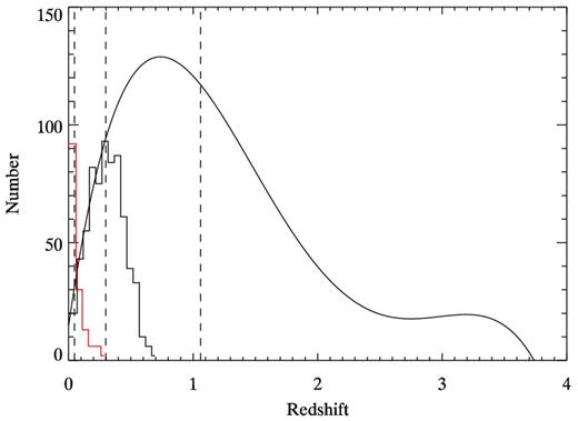
The black histogram shows the redshift distribution of radio AGN from Best & Heckman (2012), with selection as described in Section 2.2. The red histogram shows the redshift distribution of SFGs from Best & Heckman (2012). The black curve shows the redshift distribution we assume for the Kimball & Ivezić (2008) sample, which is given in de Zotti et al. (2010) and based on data from Brookes et al. (2008). The dashed lines indicate the median values for each sample.
The Best & Heckman (2012) sample has the twin advantages of providing redshifts and of differentiating between SFGs and AGNs. It is, however, much smaller than samples drawn from radio surveys without optical IDs and confined to relatively low redshifts. To also exploit the full statistics of the sensitive radio surveys and to, albeit coarsely, investigate evolution with redshift, in Section 4 we study a sample drawn from a combined cross-matched catalogue2 of Kimball & Ivezić (2008). Because this sample is not restricted to radio sources matched to galaxies in SDSS, it extends to higher redshift. From this catalogue, we use all FIRST detections falling within the region of overlap with the ACT survey that are assigned at least one match to an NVSS source. Matches are required to lie within 30 arcsec of one another. Should there be multiple FIRST or NVSS sources within the 30 arcsec matching radius, we use only the highest ranked match as per the matching algorithm detailed in Kimball & Ivezić (2008). For the stacking analysis, we use the source locations from FIRST, which are measured at high astrometric precision by the survey's 5 arcsec FWHM beam. In our subsequent modelling of these sources, we use their associated NVSS flux density measurements. The larger 45 arcsec FWHM beam of NVSS is less prone to resolving out flux density from extended sources and thus provides more accurate 1.4 GHz flux densities, as well as being a closer match to the ACT beam. To avoid stacking on lobes of extended sources that are identified as separate sources in the FIRST catalogue and more generally to avoid double counting sources that fall within a single ACT beam, we exclude sources that have neighbouring sources within 1 arcmin. This leaves 9436 sources within the overlapping FIRST and ACT observing regions (∼339 square degrees; 305° ≤ α ≤ 58°, −1| $_{.}^{\circ}$|5 ≤ δ ≤ 1| $_{.}^{\circ}$|5). We restrict the sample to the 4563 sources that have 5 < S1.4 < 200 mJy. Because we model the average SED of these sources with an AGN model, we want to remove SFGs from the sample. We mask any of these sources that lie within 5 arcmin of SFGs from the catalogue of Best & Heckman (2012). This eliminates 211 sources from the sample. The expected number of SFGs for this sample is 140 (for comparison, 149 SFGs were identified in Best & Heckman 2012), as calculated using 1.4 GHz count models based on luminosity functions from Dunlop & Peacock (1990) and Sadler et al. (2002). For the remaining sources, assumed to be radio AGN, we adopt the redshift distribution from de Zotti et al. (2010) (which was fit to data from Brookes et al. 2008) when modelling the SED. This distribution is shown in Fig. 1 and has a median redshift of 1.06 (compared to 0.30 for the Best & Heckman 2012 sample).
Sources with ACT flux density greater than three times the rms noise level of the map in any of the three bands are identified and excluded from the stacking analyses. Because the noise is determined locally, the flux density at which these cuts are drawn varies with position in the map, but typical values for the flux density threshold are 6 mJy at 148 GHz, 9 mJy at 218 GHz, and 18 mJy at 277 GHz. These sources represent outlier objects that are likely bright based on orientation, such as blazars (Urry & Padovani 1995) or based on chance alignments, such as rare, lensed SFGs (Negrello et al. 2010; Vieira et al. 2010; Marsden et al. 2014). By removing these millimetre bright sources, we reduce known inclination and lensing dependent selection effects present in a small subset of the sources. Similarly, negative 3σ deviations from the mean flux density in either band are also excluded, which will exclude large galaxy clusters with SZ decrements at 148 GHz and reduce the bias potentially introduced by excluding positive deviations in flux density from the mean. These cuts based on the ACT flux densities exclude 219 (4.8 per cent) radio sources from the stacking analysis of the Kimball & Ivezić (2008) sample and 23 (3.3 per cent) AGN from the Best & Heckman (2012) sample.
The synchrotron emission from radio-loud AGN is known to be variable. The FIRST, NVSS and ACT surveys were not simultaneous, so variability could affect the inferred spectral indices. Because the radio sources were selected based on their 1.4 GHz flux densities, variability would preferentially bias the 1.4 GHz flux density high relative to the 148 and 218 GHz flux densities, effectively steepening the average spectral index. However, the 1.4 GHz selected sources do not tend to vary as much as sources selected at ACT frequencies (which are more likely to be highly variable blazars, e.g. Marriage et al. 2011). For example, Thyagarajan et al. (2011) look for variability within the FIRST data, using three potential criteria to determine variability: the distribution of the peak flux density at different times deviates significantly (>5σ) from a normal distribution, the maximum deviation of the peak flux density from the mean exceeds 5σ, and the largest variation between data points on a light curve exceeds 6σ. They find that for FIRST radio sources with counterparts identified as SDSS galaxies, the fraction that is variable at 1.4 GHz is 0.6 per cent; the corresponding fraction for FIRST sources matched to SDSS quasars is 1 per cent.
Infrared data
We investigate the ensemble SED properties of these AGN by calculating the median flux densities at their positions across a wide range of multiwavelength data sets. To investigate the contribution of dust to the SED of the radio sources, we take advantage of surveys conducted by the Herschel Space Observatory (Pilbratt et al. 2010) using the Spectral and Photometric Imaging REceiver instrument (SPIRE; Griffin et al. 2010) that overlap with the ACT survey region: Herschel Multi-Tiered Extragalactic Large-Mode Survey (HeLMS), which is part of the Herschel Multi-Tiered Extragalactic Survey (HerMES; Oliver et al. 2012), and the publicly available Herschel Stripe 82 Survey3 (HerS; Viero et al. 2014).
SPIRE has three bands, centred at approximately 500, 350 and 250 μm (corresponding to 600, 857 and 1200 GHz, respectively). The maps used are made with SANEPIC (Patanchon et al. 2008). Of the radio-loud AGN in the ACT region from Best & Heckman (2012), 384 (58 per cent) fall within the HerS or HerMES survey regions, as do 80 SFGs (54 per cent). Of the radio sources in the sample from Kimball & Ivezić (2008), 2123 fall within the HerS or HerMES survey regions.
Flux density measurements
At 1.4 GHz, we use the catalogued NVSS flux densities corresponding to the Best & Heckman (2012) and Kimball & Ivezić (2008) sources. Data from the Parkes-MIT-NRAO survey4 (PMN; Griffith & Wright 1993; Tasker et al. 1994) and a GBT survey (Condon et al. 1994) at 4.85 GHz provide an additional constraint on the ensemble radio spectral index. For PMN and GBT as well as the Herschel surveys, we measure the flux densities in the map of each survey at the source positions, which correspond to the positions of the optical counterparts for Best & Heckman (2012) and to the positions of FIRST sources for Kimball & Ivezić (2008).
For the ACT data, as discussed in Marriage et al. (2011), given the form of the filter, the source-centred value of the filtered map multiplied by the solid angle of the beam is the source flux density. To calculate the flux densities from the map, ACT pixel values are corrected by a factor that accounts for averaging of the instrument beam peak over the 0.5 arcmin-square pixel of the ACT maps. This correction factor is applied to account for the fact that measured flux density depends on the location of a source within a pixel. For example, a source will have a lower measured flux density if it is located at the junction of two pixels instead of the centre of a pixel. We make no effort to correct this miscentring effect on a source-by-source basis, as the associated per-source dispersion is much lower than the rms noise level and averages down to a negligible level in the stack. Instead we apply an average correction given that any source has equal probability of falling anywhere within the 0.5 arcmin-square pixel. These factors correspond to 1.06 at 148 GHz, 1.10 at 218 GHz and 1.14 at 277 GHz.
We performed null tests by calculating the weighted average flux densities of randomly selected, source-free locations within the ACT+FIRST overlap region in all three ACT frequency bands. These were computed in the seven flux density bins used in Section 4 for 1000 trials of 4344 samples each. These null tests were found to be consistent with no signal with a χ2 of 5.7, 11.3 and 3.4 at 148, 218 and 277 GHz, respectively, each with 7 degrees of freedom. The corresponding probability of a random realization to exceed the observed 148, 218 and 277 GHz χ2 estimates are 0.57, 0.13 and 0.85, respectively.
Details on the stacking and uncertainty estimation for our analysis of the Best & Heckman (2012) sample and of the Kimball & Ivezić (2008) sample are provided in Sections 3 and 4, respectively.
SPECTRAL ENERGY DISTRIBUTION CONSTRUCTION AND MODELLING
In this section, we investigate the median SED for the Best & Heckman (2012) sample (with selection described in Section 2.2), which has spectroscopic redshift measurements (median z = 0.30) and was categorized into populations of AGN and SFGs. In this section, we model each of these populations independently.
Stacked flux density measurements
The SED models (described in Sections 3.2.1 and 3.3.1) were fit to the median of the flux densities (calculated as described in Section 2.4) for each band. The distribution of the flux densities of the sources (particularly at 1.4 GHz) is very broad, so we use the median flux densities in each band in order to lessen the influence of bright outliers. For each source in the Best & Heckman (2012) catalogue, we use all data available. Some sources lie outside the footprints of the Herschel surveys but fall within the ACT survey region, and we include their radio and millimetre flux densities in this analysis. Thus, the IR median flux densities are drawn from a smaller sample of sources than the radio and millimetre median flux densities, but all sources are drawn from the same parent sample, with the IR sample restricted only by sky area, so selection differences should not be significant. Indeed, the radio and millimetre median flux densities of the full sample are consistent within 1σ with the median flux densities of the subsample that lie within the Herschel survey areas. The IR surveys were treated as interchangeable, as the median flux densities for radio AGN in HerS are within the 1σ uncertainties of the median flux densities of radio AGN in HerMES for each Herschel band.
Radio-loud AGN
AGN spectral energy distribution model
The SZ spectral distortion described in equation (2) is attributed to the hydrostatically supported ionized gaseous halo around the AGN. There may be an additional SZ signal associated with a non-radiating relativistic plasma inside of ‘cocoons’ (e.g. observed as X-ray cavities in galaxy clusters) formed by the AGN during radio-mode feedback. The hypothesis of such a relativistic plasma is motivated by the fact that the minimum non-thermal pressure associated with the relativistic electrons sourcing the observed synchrotron from the cocoons is estimated to be an order of magnitude too small to be in hydrostatic equilibrium with the surrounding X-ray emitting gas (e.g. Blanton et al. 2001; Ito et al. 2008). The spatial extent of the cocoon (R < 50 kpc) is significantly smaller than the extent of the ionized gaseous halo, but the cocoon's gas pressure will likely be on average higher and the spectral distortion different from that of the non-relativistic SZ effect of the larger host halo. The formation of a cocoon may be modelled analytically as a point explosion (Ostriker & McKee 1988) using self-similar solutions to describe shock motion and associated gas state parameters (Sedov 1959). With this or other models of the cocoons, the spectral distortions of the CMB by the associated relativistic plasma (Wright 1979) inside the cocoons can then be calculated (e.g. Yamada, Sugiyama & Silk 1999; Platania et al. 2002; Pfrommer, Enßlin & Sarazin 2005; Chatterjee & Kosowsky 2007). These calculations, together with simulations (e.g. Chatterjee et al. 2008; Scannapieco, Thacker & Couchman 2008; Prokhorov, Antonuccio-Delogu & Silk 2010; Prokhorov et al. 2012), imply a signal in many systems that falls significantly below that of the SZ effect from the bulk of the non-relativistic gas of the halo and below the sensitivity of the current data. Prokhorov et al. (2010) suggest that high pressure cocoons in high-redshift systems could produce an SZ effect at 217 GHz corresponding to flux densities greater than 1 mJy. Our results rule out the possibility that such high pressure systems characterize the average SED of radio-loud AGN. Beyond this observation, we do not attempt to put constraints on SZ from the hypothesized non-radiating relativistic plasma inside cocoons and instead attribute all the SZ effect in our model to the non-relativistic gaseous atmospheres. As shown in Section 3.2.2, this model is a good fit to the data given their current precision.
We parametrize our model using the measured amplitude of the SZ effect at 148 GHz, which we call ASZ. In order to use the same parameter to model the 277 GHz data, we take into account the SZ effect frequency dependence defined according to equation (2) as well as apply a beam (and therefore band) dependent correction factor that arises due to the effect of the filter transfer function. This correction factor is discussed in detail in Appendix A. For the Best & Heckman (2012) sample, we calculate this correction factor to be 15 per cent (for comparison, the effective uncertainty on the calibration for the 277 GHz data is 15 per cent).
Results of fitting the median AGN spectral energy distribution
For the radio-loud AGN, we fit for the following parameters of the model outlined in Section 3.2.1: the radio spectral index (α), the amplitude of the SZ effect at 148 GHz (ASZ), the typical bolometric IR luminosity of the dust component expressed in solar units (log10(LIR/L⊙)), and a normalization parameter for the synchrotron emission. The best-fitting parameters are listed in Table 1. The uncertainties quoted correspond to the 68 per cent confidence intervals returned by the MCMC for each parameter. Fig. 2 shows the median flux densities for each band with the best-fitting model. The χ2 for the best-fitting AGN model is 5.8, with 4 degrees of freedom.
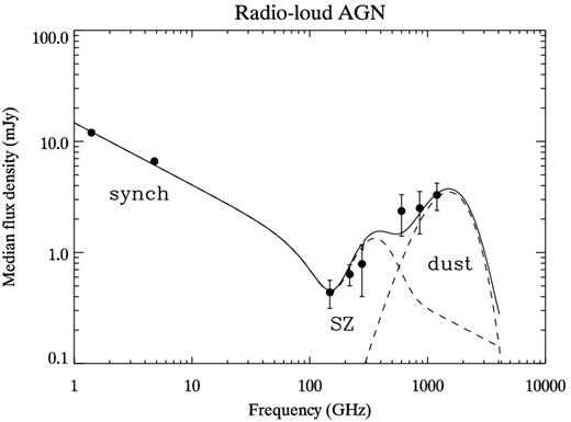
The median flux densities in NVSS, PMN/GBT, ACT and Herschel surveys of radio AGN from Best & Heckman (2012). As described in Section 3.2.1, a model with synchrotron, SZ effect and dust components is fitted to the AGN data, and the model parameters describing the best fit (shown here) are listed in Table 1. The dashed lines illustrate the synchrotron plus SZ effect component of the model and the dust grey body component of the model, and the solid line illustrates the full model evaluated for the best-fitting parameters. The error bars on the medians shown are the diagonal elements of the covariance matrix computed via bootstrap sampling (off-diagonal elements were included for the fitting). Some of the error bars are smaller than the size of the symbols. The χ2 of the fit is 5.8, with 4 degrees of freedom.
Best-fitting parameters for median AGN SED.
| α | 0.55 ± 0.03 |
| ASZ | 0.45 ± 0.13 mJy |
| log10(LIR/L⊙) | 8.7 +0.1/−0.3 |
| Ssync | 12.2 ± 0.5 mJy |
| α | 0.55 ± 0.03 |
| ASZ | 0.45 ± 0.13 mJy |
| log10(LIR/L⊙) | 8.7 +0.1/−0.3 |
| Ssync | 12.2 ± 0.5 mJy |
Best-fitting parameters for median AGN SED.
| α | 0.55 ± 0.03 |
| ASZ | 0.45 ± 0.13 mJy |
| log10(LIR/L⊙) | 8.7 +0.1/−0.3 |
| Ssync | 12.2 ± 0.5 mJy |
| α | 0.55 ± 0.03 |
| ASZ | 0.45 ± 0.13 mJy |
| log10(LIR/L⊙) | 8.7 +0.1/−0.3 |
| Ssync | 12.2 ± 0.5 mJy |
As evident in Fig. 2, the IR data constrain the dust contribution to the millimetre region of the spectra to lie below the detected median ACT flux densities for the radio AGN. There is 3σ level evidence that the SZ effect contributes to the shape of the spectrum in the ACT frequencies. If we set the ASZ term to 0, the χ2 is 16.0, with 5 degrees of freedom. The value and significance of ASZ are robust to changes in the assumed dust temperature (T = 10, 15, 20, 30 K were tested) and β (β = 2.0, 1.8, 1.5, 1.0, 0.5 were tested). We re-evaluated the best-fitting parameters for each set of T, β listed and found that for any of the models within this parametrization, the best fit ASZ is within 0.5σ of the quoted value. The best-fitting value for log10(LIR/L⊙) is not robust to changes in β and T, but increases both with increasing β and with increasing T, with T having a larger effect for the range of values probed.
We have also experimented with models that do not involve an SZ effect signal, but rather attempt to fit the data by altering source spectra. Unfortunately, few data sets constrain the spectral behaviour of large samples of radio sources at these frequencies. The Planck mission constrains the millimetre-wavelength SEDs of very bright (for example, matched to sources with S20 > 300 mJy) radio blazars (Planck Collaboration 2011c) and finds some evidence for spectral steepening. Although we exclude such sources from this analysis, we nonetheless consider a model with a spectral index change of −0.5 at 70 GHz and allow the spectral index of the dust re-emission (β) to take on values that produces a minimum χ2. For this model, β = 0.9 produces the best fit, but the resulting χ2 is 9, compared to the χ2 of 5.8 for the baseline model (with no spectral steepening, β set to 1.8, and a term for the SZ effect amplitude). When β is set to 1.8, which is typical for nearby galaxies (Smith et al. 2013), the resulting χ2 is 11. However, the synchrotron spectral behaviour for the bright Planck sources, which consist mostly of blazars, differs significantly from the average spectral behaviour of the sources in our sample. To allow more flexibility in the synchrotron shape, we adopt a model where we fix the dust spectrum β to be 1.8 and the SZ effect contribution to be 0, but introduce parameters for the location of the break in the synchrotron spectrum (νbreak) and the amount of steepening (δα, defined such that α(ν > νbreak) = α + δα). The best-fitting model values for α, δα, and νbreak are 0.47 ± 0.05, 0.2 +0.3/−0.5 and ∼4 GHz, respectively. The location of the break, νbreak, is not well constrained. The χ2 value is 5.8, with 3 degrees of freedom. If we re-introduce the SZ effect term, ASZ, into the model and fix νbreak to be 5 GHz, the resulting best-fitting parameters for α, δα and ASZ are 0.48 ± 0.04, 0.16 ± 0.08 and 0.3 ± 0.15, respectively. The χ2 is 1.3, with 3 degrees of freedom. Thus, even with this flexibility, a model with SZ is preferred, although with much lower significance than for a model with a single synchrotron spectral index. Although this model does provide a better fit than our fiducial model, the location of the spectral break at 5 GHz is not well motivated physically. When we investigate this for the larger Kimball & Ivezić (2008) sample in Section 4.3, we again find that the model including the SZ effect is preferred, and more robustly. For that sample, spectral steepening is not preferred, and a spectral break at 5 GHz is particularly unlikely (see Fig. 6).
SFG spectral energy distribution
SFG model
In addition to these sources of continuum emission, we expect that the 218 GHz band will contain some contribution from the CO J(2 − 1) spectral line at 230.5 GHz. The redshift distribution of the SFGs spans from 0.010 to 0.283 (see Fig. 1), with median redshift of 0.047. The ACT 218 GHz band is 17.0 GHz wide, with central frequency at 219.7 GHz (Swetz et al. 2011). Approximating the band transmission as a step function, for sources in the range 0.01 < z < 0.09, the CO line will fall within the ACT band. This corresponds to 80 per cent of the SFGs in the sample that fall within the ACT survey region. The true contribution of the CO line to the average SED depends on the detailed shape of the band transmission. In order to include the CO line in the SED model, we have added a parameter for additional flux density in the 218 GHz band. As a result, the 218 GHz data do not constrain the SED continuum, although obtaining a reasonable value for the CO flux density contributed can indicate consistency.
SFG modelling results
The SED model was fit to the median of the flux densities of the SFGs for each band as described for the AGN in Section 3.2.1. We fit for the following parameters of the model outlined above: the radio synchrotron spectral index (α), a normalization parameter for the synchrotron emission at 1.4 GHz, the emission measure of the free–free emission (EMff), the additional flux density at 218 GHz attributed to CO line emission (SCO), and the typical bolometric IR luminosity of the dust component expressed in solar units (log10(LIR/L⊙)). Best-fitting parameters are listed in Table 2, and the best-fitting model is shown with the median flux densities in Fig. 3. The χ2 for the best-fitting SFG model is 4.5, with 3 degrees of freedom. As with the AGN model, the covariance includes both measurement uncertainty and intrinsic variation in the flux densities.
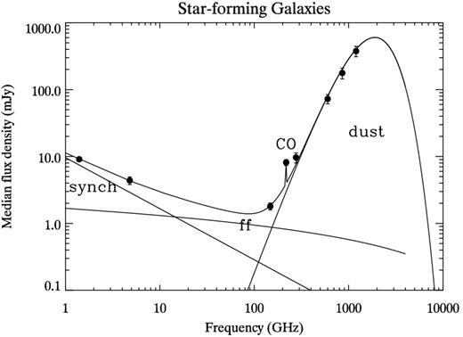
The median flux densities in NVSS, PMN/GBT, ACT and Herschel surveys of SFGs from Best & Heckman (2012). Described in Section 3.3.1, a model with synchrotron, free–free, the CO line for z = 0.05 (rest-frame frequency 230.5 GHz) and dust grey body emission is fitted to the SFG data, and the model parameters describing the best fit (shown here) are listed in Table 2. The dashed lines illustrate the synchrotron component, the free–free emission component and the dust grey body component of the model, and the solid line illustrates the full model evaluated for the best-fitting parameters. The error bars on the medians shown are the diagonal elements of the covariance matrix computed via bootstrap sampling (off-diagonal elements were included for the fitting). The error bars on the low-frequency median flux densities are smaller than the size of the symbols.
Best-fitting parameters for median SFG SED.
| α | 0.9 +0.5/−0.4 |
| Ssync | 5.5 +0.7/−0.6 mJy |
| EMff | 943 +245/−308 cm−6 pc |
| SCO | 2.8 ± 0.8 mJy |
| log10(LIR/L⊙) | 9.13 +0.07/−0.09 |
| α | 0.9 +0.5/−0.4 |
| Ssync | 5.5 +0.7/−0.6 mJy |
| EMff | 943 +245/−308 cm−6 pc |
| SCO | 2.8 ± 0.8 mJy |
| log10(LIR/L⊙) | 9.13 +0.07/−0.09 |
We can compare the best-fitting values of the median SFG SED to published models for nearby SFGs in the literature. Peel et al. (2011) use Planck data to constrain the SEDs of M82, NGC 253 and NGC 4945. They fit for more parameters than our data can constrain (particularly for the grey body spectrum, such as the dust temperature and β). Comparing with their results provides a consistency check. The emission measures they quote for their best-fitting model are 920 ± 110 cm−6 pc for M82, 284 ± 17 cm−6 pc for NGC 253 and 492 ± 81 cm−6 pc for NGC 4945. Our ensemble value of 943 +245/−308 cm−6 pc is in agreement with M82. Their best-fitting synchrotron spectral indices range from 1.1 ± 0.1 to 1.6 ± 0.4, and our value of 0.9 + 0.5/−0.4 also agrees well. Degeneracy between α and EMff is expected such that steeper values of α imply higher values of EMff, and this degeneracy is observed in the MCMC posterior distribution of those parameters. Including data for more bands at low frequency would better constrain these parameters.
We can also compare the CO line flux density with expectations from the literature. Bayet et al. (2006) measure the flux density of the CO J(2 − 1) line for nearby starburst NGC 253. Scaling by the square of the luminosity distances, the CO J(2 − 1) flux density at the median SFG redshift would be 36 mJy. NGC 253 is a bright starburst, so its CO line flux density is likely brighter than that of typical SFGs. The gas density of SFGs correlates with the star formation rate through the well-known Kennicutt–Schmidt relation (Schmidt 1959; Kennicutt 1998). Genzel et al. (2010) find a linear relation between the CO luminosity and the FIR luminosity for SFGs. If we scale the flux density by the ratio of the bolometric luminosity of NGC 253 (Rice et al. 1988) to the bolometric IR luminosity best fit to the SFG median SED, the expected CO flux density implied is 3.6 mJy, which lies within 1σ of the best-fitting CO flux density contribution to the SED.
MILLIMETRE WAVELENGTH BEHAVIOUR FOR DIFFERENT RADIO SOURCE FLUX DENSITIES
In this section, we investigate how the SEDs of the radio sources relate to their 1.4 GHz radio source flux density by binning the sample from Kimball & Ivezić (2008). This sample is much larger than that used in Section 3, but it lacks optical counterparts and thus lacks individually measured spectroscopic redshifts and classification as AGN or SFGs. This sample also extends to higher redshift (Fig. 1), enabling a comparison of properties of a low-redshift sample (discussed in Section 3) and a higher redshift sample.
Stacked flux density measurements
We compute the mean of the flux densities, which are calculated as described in Section 2.4, corresponding to subsets of sources from the Kimball & Ivezić (2008) radio source catalogue (with selection described in Section 2.2). First, we logarithmically bin sources by their associated 1.4 GHz NVSS flux density (S1.4) into 7 bins with centres ranging from 6.4 to 149.1 mJy. Then, for each source within a flux density bin, we determine the ACT flux density and the number of ACT observations at the FIRST position of the source, which determines the noise in any given pixel (see Marriage et al. 2011). Weighted by the number of observations, the ACT 148, 218 and 277 GHz flux densities (S148, S218 and S277, respectively) are then averaged to give the stacked ACT flux density for each 1.4 GHz flux density bin. Weighted averages are similarly calculated for the GBT/PMN data and Herschel, with the weights defined as the inverse of the square of the uncertainties on the flux density measurements. For the Herschel surveys, which do not cover the entire region of sky used in the ACT analysis (2123 out of 4344 of the radio sources used in this analysis lie within Herschel survey footprints), we combine all of the sources across 1.4 GHz flux density bins, calculating a single ensemble averaged flux density for each Herschel band. Constraining a single dust component also has the benefit that we do not need to know the redshift distribution of sources as a function of their 1.4 GHz flux densities and can model the full population as has been studied in the literature.
The distribution of ACT stacked flux densities within each bin was investigated via a Monte Carlo bootstrap analysis, resampling the flux density distribution with replacement for 1000 trials. We use the weighted averages of the observed sample flux densities, and we adopt the uncertainties based on the bootstrap samples. For the modelling in Section 4, we only include the covariance from the calibration uncertainties calculated in Section 2.1.1 and not bootstrap sampled covariance because we bin by 1.4 GHz flux density, which limits the amplitude of the cross-frequency-band sample covariance relative to the dominant noise in the map (unlike in Section 3.2.1, which includes sources across the full range of 1.4 GHz flux density).
Table 3 lists the results of stacking the PMN/GBT, ACT and Herschel data at the FIRST source locations for the radio source sample from Kimball & Ivezić (2008). Thumbnails of the stacked ACT data for each 1.4 GHz flux density bin of the Kimball & Ivezić (2008) sample are shown in Fig. 4. Fig. 5 shows the stacked ACT flux densities at 148, 218 and 277 GHz. The stacked ACT flux densities associated with the FIRST sources are detected at ≥3σ significance at 148 and 218 GHz for all but the highest 1.4 GHz flux density bin. The stacked ACT flux densities typically lie between 0.2 and 2.0 mJy. The faintest 1.4 GHz flux density bin contains 1767 sources and the brightest contains just 61 sources.
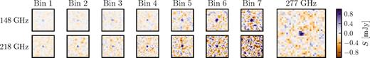
Thumbnail images (0| $_{.}^{\circ}$|25 × 0| $_{.}^{\circ}$|25) of filtered ACT data stacked on FIRST source locations. While the 148 GHz sources fade in the lower flux density bin, the 218 GHz sources remain visible. The 277 GHz map is noisier, so we have shown the 277 GHz flux densities stacked for the entire sample instead of splitting it into 1.4 GHz flux bins, although we evaluate the 277 GHz stacked flux densities for each bin for use in the analysis in Section 4.2. The 1.4 GHz flux density bins used are listed in Table 3.
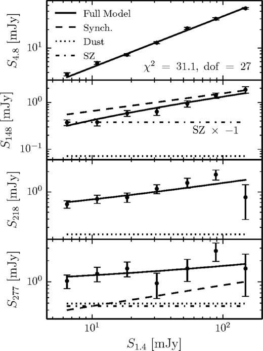
The PMN/GBT stacked flux densities at 4.8 GHz and the ACT stacked flux densities at 148, 218 and 277 GHz, with the curves corresponding to the best-fitting model and its components overlaid. The dashed line indicates the AGN emission and the dotted line indicates the contribution from dust emission. The dot–dashed line indicates SZ effect of the haloes hosting the AGN (ASZ), which is negative for ν < 218 GHz. The solid line indicates the sum of the AGN emission, the SZ effect and the dust contribution. All data are listed in Table 3.
Median flux density at radio source locations.
| Bin | S1.4 Range | Nbin | S1.4 | S4.8 | S148 | S218 | S277 | |$S_{600}^a$| | |$S_{857}^a$| | |$S_{1200}^a$| |
|---|---|---|---|---|---|---|---|---|---|---|
| (mJy) | (mJy) | (mJy) | (mJy) | (mJy) | (mJy) | (mJy) | (mJy) | (mJy) | ||
| 1 | 5.00–8.47 | 1767 | 6.43 | 3.7 ± 0.2 | 0.37 ± 0.05 | 0.66 ± 0.08 | 1.0 ± 0.2 | |||
| 2 | 8.47–14.3 | 1092 | 10.9 | 5.7 ± 0.3 | 0.38 ± 0.07 | 0.79 ± 0.1 | 1.3 ± 0.2 | |||
| 3 | 14.3–24.3 | 672 | 18.5 | 7.8 ± 0.3 | 0.59 ± 0.09 | 0.83 ± 0.1 | 1.5 ± 0.3 | |||
| 4 | 24.3–41.2 | 412 | 31.3 | 12. ± 0.5 | 0.64 ± 0.1 | 1.1 ± 0.2 | 0.96 ± 0.3 | 3.9 ± 0.4 | 4.4 ± 0.4 | 4.4 ± 0.4 |
| 5 | 41.2–69.7 | 222 | 53.5 | 21. ± 0.9 | 0.94 ± 0.1 | 1.4 ± 0.2 | 1.5 ± 0.5 | |||
| 6 | 69.7–118.0 | 118 | 88.4 | 30. ± 1.0 | 1.4 ± 0.2 | 1.8 ± 0.3 | 2.7 ± 0.7 | |||
| 7 | 118.0–200.0 | 61 | 149.0 | 45. ± 1.0 | 1.9 ± 0.3 | 0.83 ± 0.4 | 1.5 ± 0.9 |
aThe Herschel data shown correspond to a single 1.4 GHz flux density bin containing all radio sources in the sample within the Herschel survey area.
The average S148, S218 and S277 are always lower than the corresponding S1.4, as would be expected for synchrotron dominated sources with radio spectral index α1.4-148 > 0, where flux density S ∝ ν−α. However, the average S218 and S277 are greater than the average S148 for all but the highest corresponding bin in S1.4, and for most bins S277 is also higher than S218. In contrast, the synchrotron sources detected in ACT and South Pole Telescope (SPT) data, which are typically blazars and would be excluded from this analysis, tend to have flat spectral indices (∼0.2) from low frequency (1.4 or 5 GHz) to the millimetre regime, but then have falling spectral indices (α ∼ 0.5) between the millimetre bands (Vieira et al. 2010; Mocanu et al. 2013; Marsden et al. 2014). There are two possible explanations for this spectral behaviour in the stacked ACT flux densities of radio sources: either the 1.4 GHz selected sources have, on average, an inverted millimetre spectral index α148-218 < 0 and α148-277 < 0 or the SZ effect is causing the SED to rise from a decrement at 148 GHz through a null at 218 GHz to an increment at 277 GHz. We investigate each of these scenarios in the following sections, finding that the SZ effect provides a better fit to the data and thus is the preferred explanation.
Spectral energy distribution modelling
We adopt the redshift distribution based on data from Brookes et al. (2008) with the form given by de Zotti et al. (2010). The redshift distribution enters the model in the construction of the composite grey body spectrum (equation 3) and in the angular shape of the average SZ pressure profile, which affects how the SZ signal is sampled by the filter as first discussed in Section 3.2.1 and further discussed in Appendix A. For this assumed redshift distribution, the measured SZ effect at 277 GHz is 12 per cent lower than that inferred by the spectral behaviour (equation 2) and the SZ effect amplitude at 148 GHz. This correction factor is included in the construction of the model, which is parametrized by the SZ effect amplitude at 148 GHz, ASZ. Similarly, because the redshift distribution for this sample differs from that of Best & Heckman (2012), the same intrinsic amplitude of the pressure profile would produce different measurements for ASZ due to the effect of the filtering on the pressure profiles. We take this effect into account before comparing the integrated Y parameter in Section 5.1.
The CO J(2 − 1) spectral line at 230.5 GHz is not likely to contribute to the SED because for the vast majority of the sources, the redshift would place the CO line outside of the ACT band.
We perform an MCMC to determine the posterior probability distributions for the parameters α0, α1, ASZ and log10(LIR/L⊙), which are given uniform priors. We account for the full covariance of the uncertainties on the calibration and recovery of the ACT and Herschel flux densities (Section 2.1.1). Fig. 5 shows the model evaluated for the best-fitting parameters along with the data. Fig. 6 shows the resulting parameter distributions for the main parameters of interest. All chains show good convergence, with Gelman–Rubin R − 1 parameter <0.005. The best-fitting model has a χ2 = 31.1 with 27 degrees of freedom (probability to exceed = 0.27), so the model is a good fit to the data.
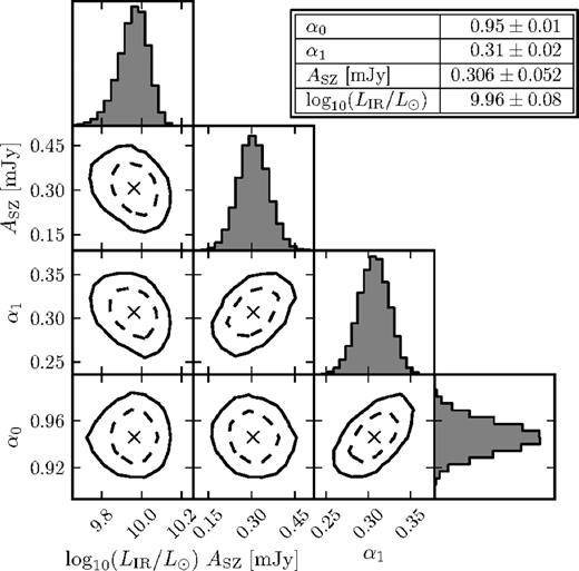
The posterior distributions of the key model parameters, with best-fitting values listed. The histograms show the single-parameter distributions for each parameter. The dashed lines show the 68 per cent confidence regions, and the solid lines show the 95 per cent confidence regions. The parameters correspond to the effective AGN spectral index at the highest 1.4 GHz flux density (α0), how the AGN spectral index varies with 1.4 GHz flux density (α1), the amplitude of the SZ from ionized gas in AGN dark matter haloes (ASZ), and the bolometric IR luminosity (log10(LIR/L⊙)).
Similarly to Section 3.2.2, we vary the dust temperature, T, and emissivity, β, of the assumed grey body dust model to determine whether our choice of T = 20 K and β = 1.8 affect our best-fitting values. For every combination of β = 1.5, 1.8 or 2.0 and T = 10, 15 or 20 K, the constraints on all parameters, with the exception of log10(LIR/L⊙), are robust to changes in these assumption (varying at the <1σ level). Moreover, the IR data strongly disfavour dust models with lower dust temperature, such that the χ2 increases by >13 for T = 15, 10 K models relative to the T = 20 K model for the ranges of β tested.
The parameter estimates from this analysis shed light on AGN and the SZ effect from radio-loud AGN hosts. Fig. 7 shows the best-fitting model for α (equation 6) and the amplitude of the SZ effect, along with the measured values for each 1.4 GHz flux density bin. The SZ effect associated with AGN hosts ASZ = 0.306 ± 0.052 mJy is detected with 5σ confidence. This level of SZ is consistent with expectations given other SZ measurements of low-mass systems and the estimated mass of the host haloes of radio-active AGN. The data are well fitted by an SZ effect term that is constant for all 1.4 GHz flux density bins. See Section 5 for further discussion of these results, including a comparison of the SZ effect measured for this sample with that measured for the Best & Heckman (2012) sample.
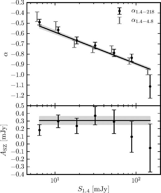
Top: the effective 1.4 GHz millimetre spectral index for each 1.4 GHz flux density bin (points), compared to the best-fitting model (solid line), for which the slope and normalization are fit. Bottom: the amplitude of the term that models the SZ signal associated with AGN, compared to the best-fitting model, which is constrained to be a constant with 1.4 GHz flux density. In both plots, the grey regions indicate the 1σ uncertainty on the best-fitting parameters of the model. For the top plot, each data point shown is calculated for a given 1.4 GHz flux density bin by solving 〈S218〉 = 〈S1.4〉(217.6/1.4)−α for α (the grey points show the equivalent for 4.8 GHz instead of 217.6 GHz). The data points shown in the bottom plot are calculated as the difference between the measured and expected 〈S148〉. For the model fit, we use the combined data set with the appropriate covariances taken into account.
The spectral index from 1.4 to 4.8 GHz is consistent with the spectral index from 1.4 to 218 GHz for sources across the full range of 1.4 GHz flux densities, as seen in Fig. 7. The AGN parameters α1, and α0 are constrained most at intermediate to high S1.4, where the SZ effect represents a smaller fraction of the flux density (though still ∼20–30 per cent) than in fainter bins. The estimated effective AGN spectral index at the highest 1.4 GHz flux density bin is 0.95 ± 0.01, consistent with optically thin, ‘steep-spectrum’ synchrotron emission, as observed in other studies. As indicated by the α1 parameter, the AGN spectral index varies with 1.4 GHz flux density such that at the lowest 1.4 GHz flux density bin (S1.4 ≈ 6 mJy), α = 0.5. This is expected for a source population composed of some flat-spectrum AGN and some steep-spectrum AGN where the relative prevalence of one population over the other varies with low-frequency flux density, as is further discussed in Section 4.3. The α = 0.55 ± 0.03 measured for the median SED of the Best & Heckman (2012) sample in Section 3.2.2 lies in the middle of the range for this model. However, for the distribution of NVSS flux densities of the Best & Heckman (2012) sample, the average expected α according to this analysis would be 0.467 ± 0.005 (statistical uncertainty from MCMC). The imposition of the requirement for optical counterparts on the Best & Heckman (2012) sample may influence the population selected such that the ensemble synchrotron spectra differ from the full radio source sample. For example, Best & Heckman (2012) preferentially exclude high-redshift galaxies, whose counterparts are not easily identifiable in SDSS. If there is some evolution in the spectra or the relative importance of flat-spectrum and steep-spectrum sources, then this could account for the differences we observe between the preferred spectral indices in the two analyses.
The best-fitting bolometric luminosity of the radio sources in this sample (log10(LIR/L⊙) = 9.96 ± 0.08) is significantly higher than the best-fitting bolometric luminosity for the lower redshift Best & Heckman (2012) sample (log10(LIR/L⊙) = 8.7 + 0.1/ − 0.3), likely indicating redshift evolution in the dust emission from the host galaxies.
Flat and steep-spectrum AGN and synchrotron spectral steepening
Because the sources in this work are selected at 1.4 GHz (and sources detected at millimetre waves are excluded), models describing populations of low-frequency sources apply to this sample more directly than those describing sources at higher frequencies. Massardi et al. (2010) model source populations from 1 to 5 GHz. As seen in previous work (de Zotti et al. 2010), they find that steep-spectrum sources dominate the 1.4 GHz source counts at all flux density levels, although with increasing contributions from BL Lac sources (characterized by flat spectra) at low flux densities ( ≲ 10 mJy) and from flat-spectrum radio quasars at high flux densities ( ≳ 500 mJy). Thus, for this paper (which only includes sources below 200 mJy), we would expect to see a population of flat-spectrum sources become more important at low 1.4 GHz flux densities, with the caveat that the spectral behaviour at high frequencies may diverge from that predicted by the counts based on studies up to 5 GHz. This population would introduce a flattening of the inferred spectral index at low 1.4 GHz flux densities. We do indeed find that the population-averaged spectral index from 1.4 GHz to millimetre frequencies is flatter at low 1.4 GHz flux densities compared to the equivalent spectral index for sources with high 1.4 GHz flux densities (see Section 4.2). Conversely, electron aging could cause a steepening of the average synchrotron spectrum, although some models predict that only the brightest blazars would tend to have such steepening at wavelengths longer than the submillimetre regime (see Ghisellini et al. 1998 for a list of references in support of and opposed to these models, see also de Zotti et al. 2010).
In order to test for the effects of spectral steepening or of the contribution from flat-spectrum sources, we introduce another parameter, Cα, defined such that α(ν > νbreak) = Cαα(ν < νbreak), where Cα can vary from −10 to 10 (and thus can capture a steepening, flattening, or inverted spectrum). We also introduce a parameter for the location of the break in the synchrotron spectrum, νbreak. The best-fitting parameters for this model are shown in Fig. 8. The location of the break in the spectrum is not well constrained by our data and tends towards the ACT frequencies. Including these new parameters does not affect the best-fitting values for any of the other model parameters: ASZ becomes 0.304 ± 0.057 mJy (5σ significance). When including the entire sample, from low 1.4 GHz flux densities to high, the best-fitting value for this new parameter is Cα = 1.05 ± 0.30. The χ2 value for the fit is 31.0 for 25 degrees of freedom (probability to exceed = 0.19), so the fit is not significantly improved by the addition of this parameter. If we only model the sources with S1.4 < 10 mJy, the value for Cα does not change significantly. The emergence of a population of flat-spectrum sources could in principle contribute to the term in our model attributed to the SZ effect at low 1.4 GHz flux densities, but this scenario is not preferred by our data when we introduce Cα. If we completely replace the SZ effect parameter from the model by this Cα parameter, the resulting χ2 = 55.3, with 26 degrees of freedom. Finally, we saw in Section 4.2 that for the model in which we include an SZ effect parameter, the average spectral index from 1.4 to 4.8 GHz agrees well with the average spectral index from 1.4 to 218 GHz for a given 1.4 GHz flux density bin, implying that the simpler model without spectral steepening adequately describes the data.
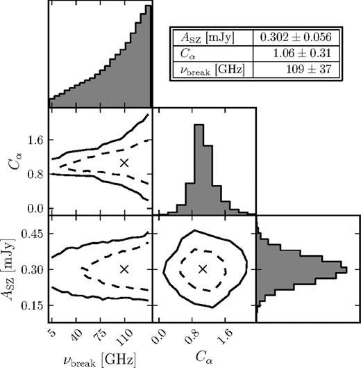
The posterior distributions of the key model parameters for the model in which the average spectra is allowed to steepen, with best-fitting values listed. The histograms show the single-parameter distributions for each parameter. The dashed lines show the 68 per cent confidence regions, and the solid lines show the 95 per cent confidence regions. The parameters correspond to the amplitude of the SZ from ionized gas in AGN dark matter haloes (ASZ), the amount by which the synchrotron spectrum index steepens (Cα), and the frequency at which the spectrum steepens (νbreak). This frequency, νbreak, is not well constrained by our data and tends to prefer a location for the steepening above the lowest ACT band at 148 GHz. The amplitude of the SZ effect is significantly non-zero even for models in which steepening is allowed.
Galaxy groups and clusters
Radio AGN occasionally reside in massive galaxy clusters and groups. To check whether the SZ effect inferred from the modelling of the data is dominated by galaxy clusters instead of arising from the more typical, lower mass environments that host most AGN, we identify and remove radio sources associated with optically selected clusters.
The Gaussian Mixture Brightest Cluster Galaxy (GMBCG) catalogue5 (Hao et al. 2010) contains more than 55 000 optically selected galaxy clusters in SDSS Data Release 7 with redshift range 0.1 < z < 0.55. While the radio source redshift distribution extends to higher redshift (see Fig. 1), we can estimate the contribution of clusters to the SZ effect signal associated with radio sources based on this lower redshift sample. Gralla et al. (2011) found that the number of radio sources per unit cluster mass does not evolve strongly with redshift. The number density of radio sources does evolve with redshift, implying that if anything the fraction of radio-loud AGN in clusters at redshifts above z ∼ 0.5 is lower than today. Thus, a significant fraction of the contribution of clusters’ SZ effect to the average SZ effect associated with radio AGN haloes should be captured by investigating these low to intermediate redshift systems.
Within the area of overlap between the ACT and FIRST surveys, there are 1903 GMBCG clusters. Comparing this subset with our 1.4 GHz sample, there were 405 sources within a 1 arcmin projected radius of a GMBCG cluster (out of 4344 total sources in the sample). Of these, only 192 would have been included in the stacking analysis; the others would have been excluded because they contain multiple radio sources. Excluding these sources near clusters from the analysis changes the S148 average values by <5 per cent, which is small compared to the errors. The model parameters (Section 4.2) are not significantly affected by the exclusion of sources that are near clusters, indicating that the ASZ term is not dominated by the richest systems.
DISCUSSION
SZ effect of radio source host haloes
As presented in Sections 3.2.2 and 4.2, there is evidence for the SZ effect from the hot atmospheres associated with the haloes hosting the radio-loud AGN at the 3σ level for the sample selected from Best & Heckman (2012) and at the 5σ level for the sample selected from Kimball & Ivezić (2008). In order to compare our results between samples and to other measurements of the SZ effect in the literature, we must convert the detected SZ amplitude to an integrated SZ signal describing the average SZ effect of the haloes hosting the radio AGN. This conversion requires an assumed angular shape of the SZ effect in order to account for its convolution with the ACT beam. For a detailed discussion of our method, assumptions and estimated uncertainties in calculating the integrated SZ signal from our measurements, see Appendix A.
For the Best & Heckman (2012) sample, we calculate an integrated E(z)− 2/3DA(z)2Y200 = 1.4 ± 0.5stat ± 0.6sys × 10− 7|$\,h_{70}^{-2}$| Mpc2, where DA is the angular diameter distance. For the Kimball & Ivezić (2008) sample, we calculate an integrated E(z)− 2/3DA(z)2Y200 = 5.4 ± 1.2stat ± 3sys × 10− 8|$\,h_{70}^{-2}$| Mpc2. The systematic uncertainties quoted include uncertainties on the profile and on the profile concentration parameter, and for the Kimball & Ivezić (2008) sample also include uncertainties in the redshift distribution of the radio sources. The integrated Y for the lower redshift Best & Heckman (2012) sample thus exceeds that of the mostly higher redshift Kimball & Ivezić (2008) sample, although at low (<2σ) significance. This may indicate evolutionary growth in the typical halo mass and associated gaseous atmosphere of radio galaxies from high redshift till today. Because the Compton parameter is integrated to θ200, it follows that the Y200 thus determined depends systematically on the mass (|$Y_{200} \propto \theta _{200}^2$| and |$\theta _{200} \propto M_{200}^{1/3}$|) due to this geometric factor. While the uncertainty on the mass is propagated through this relation to the uncertainty quoted on the measured Y200, this can also introduce a systematic uncertainty that would follow the same relation. Since we have assumed the same mass for both samples, if the high-redshift haloes have lower average mass, the underlying difference in the integrated Y between the high- and low-redshift samples would be intrinsically larger than this observed difference.
Fig. 9 shows the integrated Y parameters for both samples, with the low-redshift Best & Heckman (2012) integrated Y parameter plotted against the mass measurement for a similarly low-redshift sample from a weak lensing analysis by Mandelbaum et al. (2009). Because these measurements probe a wide range in mass and Y and for self-similar scaling Y ∝ M5/3, we also plot the mean integrated Y parameter against 〈M5/3〉3/5, which we calculate in Appendix B. If the true masses of these systems are as implied, this study has measured the SZ effect for some of the lowest mass haloes to date, as most other work investigating the stacked SZ properties of galaxies and groups targeted ∼1014M⊙ systems (Hand et al. 2011; Planck Collaboration 2011a; Sehgal et al. 2013). Planck Collaboration (2013b) probe down to a similar mass regime as we do and are also consistent with extrapolations from Y–M scaling relations based on high (galaxy cluster) mass haloes. While these previous studies bin according to mass proxy, this work computes an average value over what is likely a wide range of halo masses (see Section 5.1.1). There is good agreement among our SZ measurement for the low-redshift radio galaxies, the weak lensing and clustering mass measurement of radio galaxies similarly selected, and the measurements from Planck Collaboration (2013b) for the relation between Y and mass for local galaxies. The higher redshift Kimball & Ivezić (2008) sample integrated Y lies below the lower redshift value, possibly indicating evolutionary growth in the typical mass of radio galaxy hosts.
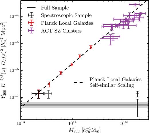
The SZ observable versus mass. The black point corresponds to the estimated integrated Y parameter that describes the SZ effect of haloes hosting radio sources in the model that best fits our data for the sample from Best & Heckman (2012), and the black error bar at the right of the plot that corresponds to this integrated Y value indicates the systematic uncertainty as estimated in Appendix A. The mass value of the black point corresponds to the average mass of haloes hosting similarly selected radio sources as determined from their weak lensing signal in Mandelbaum et al. (2009). Because the averages are calculated over a broad distribution in Y and M, and because Y ∝ M5/3 for self-similar scaling, we also indicate with a grey point the mass from Mandelbaum et al. (2009) shifted to 〈M5/3〉3/5according to expectations for the mass distributions outlined in Appendix B. The solid line indicates the estimated integrated Y parameter that describes the SZ effect of haloes hosting radio sources in the model that best fits our data for the sample from Kimball & Ivezić (2008), which has a redshift distribution that extends to much higher redshift than the sample from Best & Heckman (2012). The grey region indicates the statistical uncertainty on that measurement, and the black error bar at the right of the plot that corresponds to this integrated Y value indicates the systematic uncertainty as estimated in Appendix A. The purple data indicate the measurements for ACT SZ-detected galaxy clusters with dynamical mass measurements (Sifón et al. 2013). The red data indicate results from Planck Collaboration (2013b) from measuring the SZ effect of local bright galaxies through stacking analyses, and the dashed line indicates the scaling relation derived in that study. That the black point agrees well with the data at similar masses from Planck Collaboration (2013b) shows consistency between our measurements. The Y measurement for the higher redshift sample is lower than for the lower redshift sample, which may indicate evolution in the typical radio source host halo.
Implications for galaxy formation models
Recent observations and theory support an overall picture where most radio AGN are powered by radio-mode (or hydrostatic mode) accretion: hot gas from a hydrostatically supported halo ultimately cools and fuels the AGN, which in turn heats that gaseous halo, establishing a feedback mechanism. Our measurement of the mean SZ effect integrated Y parameter associated with radio-AGN-hosting haloes provides a direct measurement of the hot gas associated with this mechanism.
Previous studies have found that the haloes that host radio-loud AGN are indeed massive, as would be implied by this feedback scenario. For example, Mandelbaum et al. (2009) measure two-point correlation functions and galaxy–galaxy lensing shear signals to study the dark matter halo masses of radio AGN selected from FIRST and NVSS and cross-matched with SDSS. They find that the haloes hosting radio AGN are on average twice more massive than those hosting galaxies with equivalent stellar masses but without radio activity. Additionally, AGN without radio activity reside in galaxies that, as a population, have a very different distribution of stellar mass (Best et al. 2005): radio AGN reside only in galaxies above a stellar mass threshold, but optical AGN reside in galaxies both above and below that threshold. The mean mass for haloes hosting radio-loud AGN is |$(2.3\pm 0.6)\times 10^{13} \,h_{70}^{-1}$| M⊙ (for comparison, the mean mass for haloes hosting optical AGN is |$(1.1\pm 0.2)\times 10^{12} \,h_{70}^{-1}$| M⊙). Galaxy cluster BCGs are known to be preferentially radio-loud (Best et al. 2007; Lin & Mohr 2007), so Mandelbaum et al. (2009) also repeat their analysis after excluding radio AGN that lie within known optically selected clusters. While this reduces the difference between the halo masses of radio AGN and the control sample by ∼15 per cent, they still see evidence that the dark matter haloes hosting radio AGN are more massive.
Quantifying the extent to which our measurement supports the radio mode feedback paradigm requires a prediction for the average Y parameter based on the expected mass distribution for radio-loud AGN hosts. We estimate this value to be |$E(z)^{-2/3} D_{{\rm A}}(z)^{2} Y_{200} \sim 3\times 10^{-7}\,h_{70}^{-2}$| Mpc2, with details of the calculation and assumptions required given in Appendix B. The corresponding average Y for optical AGN is |$E(z)^{-2/3} D_{{\rm A}}(z)^{2} Y_{200} \sim 2\times 10^{-8}\,h_{70}^{-2}$| Mpc2, and for all galaxies is |$3\times 10^{-9}\,h_{70}^{-2}$| Mpc2. If radio emission from jets were present in all active galaxies such that they would be selected in this sample, the average halo mass of the population would correspond to an undetectable SZ effect signal given the current sensitivity and sample statistics. The fact that the measured Y is consistent with the higher mass distribution expected for radio-loud AGN provides a key consistency check of the picture that radio jets are actively providing feedback only to the most massive haloes. Even more directly, the SZ effect provides evidence for the presence of ionized gas in the haloes that host radio galaxies. We hope that the availability of this new observation will encourage the direct calculation of Y from simulations, thereby providing a new constraint for testing cosmological structure formation models with radio-mode AGN feedback.
Contribution to CMB power spectrum
Recent large millimetre surveys have enabled more sophisticated source population and spectral index modelling of high-frequency radio sources than has previously been possible (e.g. Tucci et al. 2011). In a practical cosmological context, understanding the millimetre wave spectral behaviour of radio sources is useful for modelling and removing the contribution of radio sources to high-resolution measurements of the CMB. Current experiments like Planck, SPT and ACT can use radio sources detected in their surveys to constrain the spectral indices of bright radio sources (Vieira et al. 2010; Marriage et al. 2011; Planck Collaboration 2011b; Mocanu et al. 2013). However, detected sources may also be easily masked from cosmological analyses, while faint sources that fall below the detection thresholds of these experiments still contribute to the observed power over the angular scales they probe. A better understanding of the spectral behaviour of such radio sources enables better modelling of their contribution to the power spectra and cross-power spectra for multiple frequencies (e.g. Mason et al. 2009). Characterizing the millimetre behaviour of radio sources can also be useful for SZ surveys (Lin & Mohr 2007; Lin et al. 2009; Diego & Partridge 2010; Sayers et al. 2013), as radio sources in clusters can fill in the SZ decrement at frequencies below 220 GHz.
We can also evaluate the power contributed by the SZ effect of the haloes that host radio sources and the cross-power between the SZ effect and AGN emission components. Because we bin in terms of radio source power and not SZ effect amplitude, there is the assumption that |$\langle A_{\rm SZ}^2 \rangle \sim \langle A_{{\rm SZ}} \rangle ^2$|. The SZ effect term becomes |$\ell (\ell +1)C_{\ell }^{\mathrm{SZ \times SZ}}/(2\pi ) = 0.06\pm 0.004\,\mathrm{\mu }$|K2 (statistical uncertainty) at ℓ = 3000. For comparison, Sievers et al. (2013) find that the contribution of the thermal SZ effect to the ACT CMB power spectrum at ℓ = 3000 is 3.4 ± 1.4 μK2. The cross-power term is |$\ell (\ell +1)C_{\ell }^{\mathrm{A \times SZ}}/(2\pi ) = -0.29 \pm 0.07\,\mathrm{\mu }$|K2.
CONCLUSIONS
We have investigated the ensemble millimetre properties of 1.4 GHz selected radio sources by stacking 148, 218, 277, 600, 857 and 1200 GHz data from ACT and Herschel on the positions of radio sources selected from two joint catalogues of FIRST and NVSS 1.4 GHz sources. Although most of the radio sources are AGN, whose spectra are expected to fall with increasing frequency at millimetre wavelengths, we see evidence for an average rising spectrum. This observed spectral inversion in the ACT bands is attributed to the SZ effect of the haloes that host the AGN. We construct SEDs for a sample of radio sources (Best & Heckman 2012) that have optical counterparts and thus known redshifts and classifications as either AGN or SFGs. In order to constrain the contribution to the SED from dust emission, we also stack data from Herschel surveys, and to better constrain the synchrotron spectrum we include 5 GHz data from PMN and a GBT survey. The AGN SED is well fitted by a model that includes synchrotron emission, the SZ effect and dust emission. The SFG SED is well fitted by a model that includes synchrotron emission, free–free emission, CO line emission and dust emission.
Using a larger catalogue enables the construction of SEDs for sources binned in 1.4 GHz flux density. The radio source sample from Kimball & Ivezić (2008) was constructed without optical counterparts, and while spectroscopic redshifts are lacking, the sample includes greater numbers of sources (4344 used in this study) and extends to higher redshifts. Even though we exclude bright ACT sources, the binned 1.4 GHz selected radio sources are detected in the ACT data. The ensemble averaged millimetre synchrotron spectral index (S ∝ ν−α) for AGN is 0.95 ± 0.01 for the bright (∼100 mJy) sources, with evidence for flattening towards fainter 1.4 GHz source flux densities. The best-fitting model includes an SZ contribution detected at the 5σ level.
The detection of the SZ effect in the radio galaxies’ millimetre wavelength SED provides evidence that, on average, galaxies that host radio AGN support hot gaseous haloes. This is important in the context of the growing support for the overall picture that most radio AGN are powered by radio-mode accretion, where AGN are fuelled by the accretion of gas ultimately from the hot hydrostatically supported halo. In this picture, the radio jets from the AGN in turn provide energy that counters the cooling of the gas, shutting off the AGN fuel supply by establishing a feedback loop.
We have also calculated the contribution of these radio sources to the CMB power spectrum. At 148 GHz, after correcting for the SZ effect, the sources contribute |$\ell (\ell +1)C_l^{\mathrm{A \times A}}/(2\pi )=0.37 \pm 0.03\,\mathrm{\mu }$|K2 at ℓ = 3000, where the uncertainty is dominated by the uncertainty on the contribution to the SZ effect to the measured flux densities. The cross-power between the SZ effect and the radio source emission at 148 GHz is |$\ell (\ell +1)C_{\ell }^{\mathrm{A \times SZ}}/(2\pi ) = -0.29 \pm 0.07\,\mathrm{\mu }$|K2.
This work was supported by the US National Science Foundation through awards AST-0408698 and AST-0965625 for the ACT project, as well as awards PHY-0855887 and PHY-1214379. Funding was also provided by Princeton University, the University of Pennsylvania, and a Canada Foundation for Innovation (CFI) award to UBC. ACT operates in the Parque Astronómico Atacama in northern Chile under the auspices of the Comisión Nacional de Investigación Científica y Tecnológica de Chile (CONICYT). Computations were performed on the GPC supercomputer at the SciNet HPC Consortium. SciNet is funded by the CFI under the auspices of Compute Canada, the Government of Ontario, the Ontario Research Fund – Research Excellence; and the University of Toronto. MBG and TAM acknowledge support from Johns Hopkins University. RD, PA, FR and GM received funding from the Chilean grants FONDECYT 11100147 and BASAL (CATA). This research made use of astropy, a community-developed core python package for Astronomy (Astropy Collaboration 2013).
Herschel is an ESA space observatory with science instruments provided by European-led Principal Investigator consortia and with important participation from NASA.
REFERENCES
APPENDIX A: CALCULATION OF INTEGRATED Y PARAMETER FROM MEASURED PARAMETER ASZ
To estimate a characteristic R500 for the radio AGN, we use the lensing mass estimate from Mandelbaum et al. (2009) (|$M_{200}= 2.3 \pm 0.6 \times 10^{13} \,h_{70}^{-1}$| M⊙). For R500 and other relevant quantities (e.g. angular diameter distance), we calculate medians and means based on the redshift distributions shown in Fig. 1. To use the mass estimate from Mandelbaum et al. (2009) with the UPP R500-scaled profile, we convert M200 to |$M_{500} \approx 1.5 \times 10^{13} \,h_{70}^{-1}\,\mathrm{M}_{\odot }$| assuming the dark matter follows a Navarro, Frenk & White (1997) (NFW) profile, using the concentration–mass relation from Duffy et al. (2008). Estimated in this way, |$R_{500}= 0.34\,h_{70}^{-1}\,{\rm Mpc}$| (θ500 = 1.24 arcmin) for the sample of Best & Heckman (2012), and |$R_{500} = 0.25\,h_{70}^{-1}\;{\rm Mpc}$| (θ500 = 0.64 arcmin) for the higher redshift sample of Kimball & Ivezić (2008). The redshift distribution of haloes for which Mandelbaum et al. (2009) estimated a mean M200 is best matched to the lower redshift sample of Best & Heckman (2012). Lacking a mass estimate for radio AGN-hosting haloes with the higher redshift distribution of the Kimball & Ivezić (2008) sample, we have simply used the same M200 to estimate R500 for both samples.
The angular profiles of the projected SZ effect pressure and for the ACT beams. The dashed line shows the profile assumed for the sample from Best & Heckman (2012) (median z = 0.30) and the solid line shows the profile assumed for the sample from Kimball & Ivezić (2008) (median z = 1.06). The red line shows the ACT 148 GHz beam profile and the purple line shows the ACT 277 GHz beam profile.
In order to characterize the level of additional systematic uncertainties, we varied the assumptions made in this calculation about the radio source redshift distribution, the typical pressure profile and the typical halo concentration. To estimate the 1σ systematic uncertainty contributed by each of these assumptions, we calculate the difference between the values given the alternative models described below and the values calculated using our fiducial model. To calculate a total systematic uncertainty for each sample, we add these systematic uncertainties in quadrature. If we adopt the redshift distribution of the radio sources given by Ho et al. (2008), the value for the Kimball & Ivezić (2008) sample becomes E(z)− 2/3DA(z)2Y200 = 4.5 ± 1.0 × 10⁻⁸|$\,h_{70}^{-2}$| Mpc2, which is in agreement with the value calculated above for the redshift distribution as reported by de Zotti et al. (2010). Adopting the halo concentration–mass relation from Neto et al. (2007) yields E(z)− 2/3DA(z)2Y200 = 1.5 ± 0.5 × 10⁻⁷|$\,h_{70}^{-2}$| Mpc2 for the Best & Heckman (2012) sample and E(z)− 2/3DA(z)2Y200 = 5.7 ± 1.3 × 10⁻⁸|$\,h_{70}^{-2}$| Mpc2 for the Kimball & Ivezić (2008) sample. Finally, if we adopt the best-fitting profile of Planck Collaboration (2013a), who measured the SZ pressure profiles of 62 massive, low-redshift clusters, we find a resulting value of E(z)− 2/3DA(z)2Y200 = 2.0 ± 0.7 × 10⁻⁷|$\,h_{70}^{-2}$| Mpc2 for the Best & Heckman (2012) sample and E(z)− 2/3DA(z)2Y200 = 8.7 ± 2.0 × 10⁻⁸|$\,h_{70}^{-2}$| Mpc2 for the Kimball & Ivezić (2008) sample. This pressure profile parametrization is more extended than the fiducial Arnaud et al. (2010) profile, so a given estimate of the amplitude of the signal yields a larger value for the integrated Y parameter.
In summary, we find an integrated E(z)− 2/3DA(z)2Y200 = 5.4 ± 1.2stat ± 3sys × 10− 8|$\,h_{70}^{-2}$| Mpc2 for the Kimball & Ivezić (2008) sample and an integrated E(z)− 2/3DA(z)2Y200 = 1.4 ± 0.5stat ± 0.6sys × 10− 7|$\,h_{70}^{-2}$| Mpc2 for the Best & Heckman (2012) sample.
APPENDIX B: ESTIMATED HALO MASS DISTRIBUTION FOR RADIO-LOUD AGN HOSTS
We have measured the mean integrated Compton parameter Y for hosts of radio-loud AGN. From self-similar arguments, we expect this parameter to be related to the host's halo mass M200 as |$Y_{200} E^{-2/3}(z) D_{\rm A}^2(z) \propto M_{200}^{5/3}$| (Kaiser 1986). In this appendix, we estimate the mean M200 and |$M_{200}^{5/3}$| for local (z < 0.6) radio-loud AGN hosts, corresponding to the redshift range of the spectroscopic sample (Best & Heckman 2012) used in Section 3. Schematically, this is done by using the stellar mass function for all galaxies ϕ(M*) (Cole et al. 2001) scaled by the radio-loud AGN fraction frad(M*) (Best et al. 2005) and then using an approximate functional form for the stellar-to-halo mass relation M200(M*) from lensing (Mandelbaum et al. 2009) to compute the mean M200 and |$M_{200}^{5/3}$|. A similar treatment is carried out for optically selected AGN. This allows us to approximate what mean Compton Y is expected for AGN hosts. Perhaps more importantly, it allows us to evaluate the level of correction needed in comparing the mean |$Y_{200} E^{-2/3}(z) D_{\rm A}^2(z)$|, taken over the entire AGN host population (from |$\langle M_{200}^{5/3} \rangle$|), to the mean halo mass 〈M200〉 from lensing or clustering studies, as in Fig. 9.
Stellar and halo mass distribution functions (per decade in mass) for all ‘control’ galaxies, galaxies with radio AGN and galaxies with optical AGN. The vertical lines indicate the mean mass of each distribution.
