


Abstract
Located at 2 pc, the L7.5+T0.5 dwarfs system WISE J104915.57−531906.1 (Luhman 16 AB) is the third closest system known to Earth, making it a key benchmark for detailed investigation of brown dwarf atmospheric properties, thermal evolution, multiplicity, and planet-hosting frequency. In the first study of this series – based on a multicycle Hubble Space Telescope (HST) program – we provide an overview of the project and present improved estimates of positions, proper motions, annual parallax, mass ratio, and the current best assessment of the orbital parameters of the A-B pair. Our HST observations encompass the apparent periastron of the binary at 220.5 ± 0.2 mas at epoch 2016.402. Although our data seem to be inconsistent with recent ground-based astrometric measurements, we also exclude the presence of third bodies down to Neptune masses and periods longer than a year.
1 INTRODUCTION
The first completeness-corrected planet occurrence rates emerging from the Kepler mission reveal a larger number of short-period Earth-sized planets around M dwarfs than around earlier-type (FGK) stars (Dressing & Charbonneau 2013; Fressin et al. 2013). Combined with state-of-the-art planet radius–mass relationships, studies indicate that there are about 3.5× as many 1–4 |$\mathcal {M}_{\rm Earth}$| mass planets around M-type stars than around G-type stars, with a period-dependence on planet occurrence rate that varies monotonically with host spectral types (Mulders, Pascucci & Apai 2015). The larger number of small planets around M dwarfs contains more mass in solids than the same small planet population around G-type stars (Mulders et al. 2016). Given that discs around higher mass stars have higher masses (e.g. Pascucci et al. 2016), the higher occurrence rates, and higher solid mass of small planets around lower mass stars may be the result of inward migration of planets or their planetary building blocks. The recent discovery of seven approximately Earth-sized planets in the TRAPPIST-1 system (a star at the stellar/substellar boundary) provides a striking demonstration of the high occurrence rates of small planets around small stars (Gillon et al. 2017).
These results motivate studies of the small planet population around even lower mass hosts, the brown dwarfs (BDs, Kumar 1962; Hayashi & Nakano 1963). These low-mass objects, incapable of hydrogen fusion, also host circumstellar discs (e.g. Luhman et al. 2008) which evolve through the first steps of planet formation (e.g. Apai et al. 2005; Pascucci et al. 2009; Ricci et al. 2013). However, planet detection through radial velocity (RV), transit, and high-contrast imaging are not effective for BD primaries due to their low luminosities (<10−3 L⊙; Burrows et al. 2001). In contrast, high-precision astrometric observations have the potential to provide an extremely sensitive assessment of the presence of planets and to constrain the orbital inclination of the planetary system.
The Wide-field Infrared Survey Explorer (WISE) has discovered many of the nearest BDs in the Solar neighbourhood (d < 20 pc). A key example is WISE J104915.57−531906.1 AB, identified by Luhman (2013) as a binary BD located 2 pc from the Sun (hereafter Luhman 16 AB to follow the Burgasser et al. 2013 denomination). Luhman 16 A and B orbit each other at a distance of a few astronomical unit with an orbital period of decades. As the closest known BDs, the system is ideally suited for detailed characterization.
The primary (Luhman 16 A) is of spectral type L7.5 ± 1 and the secondary (Luhman 16 B) of type T0.5 ± 1.5. Both at effective temperatures of about 1300 K, placing them near the L-T transition (Luhman 2013; Burgasser et al. 2013; Kniazev et al. 2013; Faherty et al. 2014; Lodieu et al. 2015). The system age is constrained to about 0.1–3 Gyr, implying masses below 0.06 |$\mathcal {M}_{{\odot }}$| (Faherty et al. 2014; Lodieu et al. 2015). There is no evidence for the pair belonging to any nearby young moving group (Mamajek 2013; Lodieu et al. 2015). Both BDs are known variables, with the B component more strongly variable than A. The variability likely originates from patchy clouds (Gillon et al. 2013; Crossfield et al. 2014; Buenzli et al. 2014, 2015a; Karalidi et al. 2016).
Boffin et al. (2014) reported perturbations of the A-B orbital motions in the Luhman 16 system, suggesting the presence of a third body. Later, Sahlmann & Lazorenko (2015) using the same Very Large Telescope (VLT) data and those from the follow-up monitoring programme by Boffin et al., have excluded the presence of any third object with a mass greater than two Jupiter masses orbiting around either BD with a period between 20 and 300 d.
Past- and present-day ground-based seeing-limited imaging- and adaptive-optics facilities have fundamental limitations (field of view, point spread function (PSF) stability, differential atmospheric chromatic effects, and seasonal visibility), all of which introduce systematic and seasonal astrometric errors that are difficult to quantify or isolate when constraining the presence of companions via astrometry. This is particularly true for faint and red objects, which are much redder than the stars used as reference in the field. In the case of Luhman 16, there is the additional complication of observing a tight binary system (at an average separation of ∼1″ and down to 0|${^{\prime\prime}_{.}}$|22, see the next sections). In the past, these systematic errors have resulted in false detections of planetary companions. These include reports of exoplanets orbiting Lalande 21185 (van de Kamp & Lippincott 1951; Lippincott 1960) and Barndard's star (van de Kamp 1963, 1969), both later refuted (Gatewood & Eichhorn 1973; Gatewood 1974). More recently, a giant planet was claimed to orbit the M8 dwarf VB 10 by Pravdo & Shaklan (2009) based on ground-based astrometric observations, a claim subsequently refuted by Lazorenko et al. (2011), among others. These and other examples point to the importance of high-precision – sub-milli-arcsecond (mas) – space-based astrometry for robust detection of exoplanets around very low-mass stars and BDs.
For these reasons, we have used the Hubble Space Telescope (HST) in a special mode to obtain the most accurate annual parallax of any BD to date (eventually down to the 50 μas) for each of the two components of Luhman 16, and to constrain their absolute space motions with similar accuracy. Most importantly, by searching for astrometric perturbation of the A-B orbital motion, we will be able to confirm whether giant planet candidates exist in this system uncovering exoplanets down to a few Earth masses, as described below. Our HST data could also potentially complement/extend the work done by Melso, Kaldon & Luhman (2015) searching for giant planets as resolved, faint companions comoving with the targets; however, we will see that this is not the case.
In this first article, we focus on the standard imaging analysis of our existing HST data using procedures and methods widely used in literature, sufficient to significantly improve characterization of this BD binary system. In Section 2, we detail our observing strategy. In Section 3, we describe our data reduction and measurements. We explore two methods to derive astrometric and orbital parameters, through simultaneous fit of the parameters (Section 4) and through a two-step fitting procedure (Section 5). In Section 6, we use the limited RVs for the two components available in the literature to remove the degeneracy in the sign of the orbital inclination. In Section 7, we examine the photometric variability of the sources. In Section 8, we examine the potential presence of exoplanets based on this analysis, ruling out the presence of planets more massive than one Neptune mass, and pointing out several mas-level inconsistencies between HST and existing ground-based astrometry from Sahlmann & Lazorenko (2015, hereafter SL15). In Section 9, we summarize the electronic material released as part of this work. In Section 10, we summarize our conclusions.
2 OBSERVING STRATEGY
The imaging data acquired for this project are obtained with the Ultraviolet-VISual (UVIS) channel of the Wide Field Camera 3 (WFC3) instrument on HST under programs GO-13748 and GO-14330 (PI: Bedin). UVIS has a wide field of view of about 160″ × 160″ and the best image quality on-board of HST, with two detectors of ∼4000 × 2000 pixels2, and a pixel scale of ∼39.77 mas.
The main goal of our program is to probe Luhman 16 AB for the presence of additional, yet unknown bodies, down to ∼5 Earth masses, through astrometric perturbations of the A-B orbital motion. Our observations were designed to maximize the high-precision astrometric capabilities of the HST with the relatively new cutting-edge technique of spatial-scanning mode. Spatial scanning under fine guide sensors control is an observing mode implemented for WFC3 on HST only recently, with the original aim of high-precision photometry during exoplanet transits (McCullough & MacKenty 2012). In this mode, the target field is observed while the telescope slews in a specified direction and rate. This spatial scanning enables up to thousands of times more sampling of the same sources (targets and references), boosting photometric precision over pointed imaging. In the following, we will refer to these images in spatial-scanning mode as trailed, and to those obtained in the standard mode as pointed. Recently, Riess et al. (2014) employed this newly developed HST observing mode for WFC3 also to the case of astrometry. By scanning perpendicularly to the long axis of the parallax ellipse, this mode can considerably improve the precision of parallax measurements. Riess et al. demonstrated the possibility to measure changes in a source's position to a precision of 20–40 μas. This is almost an order of magnitude better than what is attainable employing the best techniques in traditional pointed imaging with the WFC3/UVIS (i.e. 320 μas, see Bellini, Anderson & Bedin 2011). As a rule of thumb, the astrometric precision essentially scales with the length of the trails. As in point-source imaging all the weight comes from the innermost 5 pixels, therefore trailing for 2000 pixels, results in a 2000/5 = 400 times more pixels, and therefore the gain is a factor of |$\sqrt{400}=20$|. Accurate calculations are more complicated, and residuals in geometric distortion, currently calibrated down to 320 μas (Bellini et al. 2011) need to be suppressed to make this potential gain usable down to 20 μas (Casertano et al. 2016). There are important differences between our observing mode and analyses, and those proposed by Riess et al. (2014) or Casertano et al. (2016), which will be discussed in a subsequent paper analysing the trailed images.
The data for this project are collected in 13 visits at well-defined epochs, five at the maximum elongations of the parallax, and eight at fractional phases of the year at (approximate) logarithmic sampling. Sampling periods are between 30 d and 3 yr. Twelve of these visits have been collected.
The images (two-dimensional (2D) data) collected in 13 epochs provide 26 independent data points to solve for the Luhman 16 AB baricentric positions, baricentre motions, parallax, mass ratio, and for the seven parameters of the A-B orbit (13 parameters), plus detection of any significant deviation. Naturally, it would not be possible to firmly constrain the A-B orbit until at least half of the orbit will be completed, but we would still be able to firmly detect deviations from a conic arc, induced by additional bodies, at least for periods between ∼30 d up to ∼3 yr.
The roll angle (hereafter, PAV3, i.e. the position angle of axis V3 of the HST's focal plane1) was varied among the visits to minimize hidden systematic errors. Data were acquired in six different roll-angle values, with each roll angle used on at least two visits. The dither pattern within each epoch was also carefully designed. We imposed large dither steps of at least ±100 pixels to have a check on the distortion residuals. We also avoided having Luhman 16 A and B fall on any of the lithographic features or other known cosmetic defects of the two UVIS CCDs (see Bellini et al. 2011), or in the gap between the two chips. Two known extragalactic sources also fell in all images, which will be used in future works as an external check on absolute positions.
The main astrometric trailed exposures are collected in filter WFC3/UVIS/F814W. Although a medium or narrow-band filter would be better for astrometry, as PSFs would be less dependent on the colour of the targets, filter F814W has the valuable property that Luhman16 A and B have almost the same count rates. Furthermore, the F814W filter has one of the best characterized geometric distortion solutions (Bellini et al. 2011).
Future analyses of the trailed images require pointed images to characterize the sources in the patch of sky (targets and the reference stars) and colour information to trace potential chromatic dependencies. Therefore, two 60 s short-pointed exposures in F814W are also taken at the beginning and at the end of each orbit to provide an input list, where both components of Luhman 16 are just below saturation level, i.e. at the maximum astrometric signal-to-noise ratio possible. Next, to get the colour information of the sources in the field, we choose the filter WFC3/UVIS/F606W, which is sufficiently bluer than F814W, and the best compromise between depth and reasonable signal for the cool components of Luhman 16. Due to the time required by the frame buffer dump, the exposure time for an optimal duty cycle is ∼350 s. Our trailed exposures have at least this exposure times, and when visibility allows it, even longer. Therefore, in addition to the two short exposures, we could not fit more than five long exposures per orbit, of which four are trailed in F814W, and one is a pointed image in F606W. Seven exposures per orbits means that in the end there will be 52 trailed images of at least 350 s in F814W, and 39 pointed images, 26 of which of 60 s in F814W, and 13 of ∼350 s in F606W, for a grand total of 91 images. So far 12 of 13 visits have been collected, i.e. 36 pointed images are available.
This article is based – exclusively – on these pointed images, 24 in filter F814W and 12 in filter F606W. Table 1 gives information on these 36 images.
HST images used in this work (ID is not in MJD order).
| Number ID: MJDstart | Image EXPT | PAV3(°) |
|---|---|---|
| F814W | ||
| 01: 56891.03123284 | icmw09v1q 60 s | 345.010712 |
| 02: 56891.10048062 | icmw09waq 60 s | 345.006592 |
| 03: 56935.09556248 | icmw04l1q 60 s | 40.016430 |
| 04: 56935.12740285 | icmw04lcq 60 s | 40.013191 |
| 05: 57031.75281042 | icmw02zlq 60 s | 144.999603 |
| 06: 57031.82073857 | icmw02zwq 60 s | 145.003006 |
| 07: 57059.93495262 | icmw12asq 60 s | 160.003403 |
| 08: 57059.96679262 | icmw12b3q 60 s | 160.007401 |
| 09: 57115.70210654 | icmw07ccq 60 s | 215.013794 |
| 10: 57115.73394691 | icmw07cnq 60 s | 215.017197 |
| 11: 57204.00903025 | icmw01vbq 60 s | 325.005707 |
| 12: 57204.07274544 | icmw01vyq 60 s | 325.002289 |
| 13: 57255.02930926 | icmw10bsq 60 s | 345.010712 |
| 14: 57255.06114963 | icmw10caq 60 s | 345.006592 |
| 15: 57300.55774736 | icmw05dfq 60 s | 40.016430 |
| 16: 57300.59198366 | icmw05dqq 60 s | 40.013191 |
| 17: 57395.65852572 | icmw03xoq 60 s | 144.999603 |
| 18: 57395.69036609 | icmw03xzq 60 s | 145.003006 |
| 19: 57429.21396601 | icmw13uyq 60 s | 161.070297 |
| 20: 57429.28672083 | icmw13v9q 60 s | 161.074203 |
| 21: 57479.56281007 | icmw08bvq 60 s | 215.013794 |
| 22: 57479.62306489 | icmw08c6q 60 s | 215.017197 |
| 23: 57665.08973572 | icte06rvq 60 s | 40.016430 |
| 24: 57665.12157609 | icte06saq 60 s | 40.013191 |
| F606W | ||
| 25: 56891.04534173 | icmw09v8q 348 s | 345.008606 |
| 26: 56935.10967137 | icmw04l6q 348 s | 40.014809 |
| 27: 57031.76691931 | icmw02zqq 348 s | 145.001297 |
| 28: 57059.94906114 | icmw12axq 348 s | 160.005402 |
| 29: 57115.71621543 | icmw07chq 348 s | 215.015503 |
| 30: 57204.02463210 | icmw01vhq 348 s | 325.003998 |
| 31: 57255.04341815 | icmw10c2q 348 s | 345.008606 |
| 32: 57300.57305995 | icmw05dkq 348 s | 40.014809 |
| 33: 57395.67263424 | icmw03xtq 348 s | 145.001297 |
| 34: 57429.25623453 | icmw13v3q 348 s | 161.072296 |
| 35: 57479.57691896 | icmw08c0q 348 s | 215.015503 |
| 36: 57665.10384461 | icte06s3q 348 s | 40.014809 |
3 DATA REDUCTIONS AND MEASUREMENTS
In this section, we provide a brief description on how the positions in pixel coordinates (x, y) for all the stars in the individual frames were obtained, transformed into a common reference frame (X, Y), and into a standard equatorial coordinate system (α, δ) at Equinox J2000. At each step, we also give reference to works containing more exhaustive descriptions of the adopted procedures and software.
3.1 Correction for imperfect CTE
Imperfections in the charge transfer efficiency (CTE) smear the images, which result in compromised astrometry (see Anderson & Bedin 2010). In all our observations, we have mitigated the CTE effects in two ways: (1) passive CTE mitigation: we have downloaded the figlc images, which apply the pixel-based CTE correction algorithms developed for the Wide Field Channel (WFC) of the Advanced Camera for Surveys (ACS, Anderson & Bedin 2010) and are already implemented also for WFC3/UVIS images by the Space Telescope Science Institute (STScI) pipeline. They are now downloadable as standard data-products at the MAST archive.2 (2) Active CTE mitigation: we have applied a post-flashing (of about 12 e−) to keep the background above the critical threshold (filling many of the charge traps), which suppress as much as convenient the residuals due to imperfect CTE.3 However, both strategies do not work perfectly, and traces of these imperfect CTE remain. The residuals left on the measured positions are sizable (∼0.5 mas), but thankfully, they are also (relatively) easy to track down and remove (see following sections).
3.2 Fluxes and positions in the individual images
Positions and fluxes of sources in each WFC3/UVIS figlc image were obtained with software that is adapted from the program img2xym_WFC.09x10 developed for ACS/WFC (Anderson & King 2006), and publicly available.4 Together with the software, a library of effective PSFs for most common filters is also released. These are spatially variable in a 7 × 8 array, and can also be perturbed in a spatially constant mode to better fit PSFs of individual frames. However, we follow the Bellini et al. (2013) prescription to perturb the library PSFs also spatially (in a 5 × 5 spatial array). These procedures tailor the library PSFs to each individual image even better than spatially constant perturbed PSFs, as they better account for small focus variations across the whole field of view. In addition to solving for positions and fluxes, the software also provides a quality-of-fit parameter (Q). The quality of fit essentially tells how well the flux distribution resembles the shape of the PSF (this parameter is defined in Anderson et al. 2008). It is close to zero for stars measured best. This parameter is useful for eliminating galaxies, blends, and stars compromised by detector cosmetic or artefacts.
Once the raw pixel positions (xraw, yraw) and magnitude are obtained, they are corrected for geometric distortion. We used the best available average distortion corrections for WFC3/UVIS (Bellini & Bedin 2009; Bellini et al. 2011) to correct the raw positions and fluxes of sources that we had measured within each individual image. (Note that fluxes are also corrected for pixel area using the geometric distortion correction). We refer to corrected positions in the individual frame with the symbols (xcor, ycor).
Finally, we note that given the large width of the filter passband of F606W and F814W, the PSFs for very red stars are significantly different from the PSFs of average colour stars in the field. This fact is evident in the relatively large values of Q for Luhman 16 A and B, compared to stars of similar magnitudes; and residuals in the subtracted images of Luhman 16 A and B. These fit mismatches could potentially lead to chromatic systematic errors in positions, known to affect UV filters (Bellini et al. 2011). However, as described below, such offsets are below the level of other systematic errors (i.e. ∼320 μas for geometric distortion) for this analysis.
3.3 The reference frame
As our reference frame we adopted the best-fitting (∼200) stars measured in the first exposure of our first epoch. These stars were unsaturated, with at least 4000 e−, isolated by at least 9 pixels, and with Q < 0.4. To avoid negative values when stacking all images from all epochs (see the next section), we added 1000.0 pixels in each coordinate to the distortion-corrected positions of these stars; the resulting coordinates are indicated with (X, Y) and are the positions in our adopted reference frame. We then find the most general linear transformation (six parameters), between the distortion-corrected positions of these stars of the reference frame (X, Y), and their distortion-corrected positions (xcor, ycor) in any other image (for as many stars in common as possible). This enables us to perform all of the relative measurements with respect to this reference frame. These transformations were computed using only stars with positions consistent to at least 3.6 mas (or 0.09 pixels). This ensured that we use only stars that are present in all imaging epochs and do not have compromised measurements due to cosmic rays or detector cosmetics. The underlying assumption is that stars in the field have negligible common and peculiar motions; however an uncertainty of 3.6 mas on ∼200 stars still leads to an uncertainty of 250 μas on the centroid position. In this work, we will not attempt to iteratively solve for the motions of individual reference field objects, as again, these uncertainties are of the same order of the precision of the astrometry in pointed images. We will see in Section 3.4 how this positional precision is consistent with Gaia data-release (DR1) positions.
For the same reasons, and differently from the more sophisticated local-transformations procedure described in Bedin et al. (2014), we do not apply any local approach, due to the relatively low stellar density in the field, and as our final residuals using global transformations are already consistent with our expected uncertainties.
The observed positions in the (X, Y) reference frame for Luhman 16 A and B in the 36 pointed images analysed in this work are given in Table 2. There, we also give the (xraw, yraw) positions which will be used to track down the systematic effects of residuals of imperfect CTEs, and to correct for them.
Observed positions for Luhman 16 A and B in both the master frame coordinate system and in the raw coordinate system of the individual images. The ID is as in Table 1.
| Number ID | |$X_{\rm A}^{\rm obs}$| | |$Y_{\rm A}^{\rm obs}$| | |$x_{\rm A}^{\rm raw}$| | |$y_{\rm A}^{\rm raw}$| | |$X_{\rm B}^{\rm obs}$| | |$Y_{\rm B}^{\rm obs}$| | |$x_{\rm B}^{\rm raw}$| | |$y_{\rm B}^{\rm raw}$| |
|---|---|---|---|---|---|---|---|---|
| 01 | 3177.4275 | 4480.9977 | 2180.594 | 3248.659 | 3200.5454 | 4483.9296 | 2203.846 | 3249.985 |
| 02 | 3177.4303 | 4481.0021 | 2382.559 | 3031.726 | 3200.5414 | 4483.9315 | 2405.762 | 3033.062 |
| 03 | 3176.9366 | 4479.5016 | 2884.488 | 2699.714 | 3198.7634 | 4481.8825 | 2898.892 | 2682.114 |
| 04 | 3176.9435 | 4479.5022 | 3084.968 | 2484.191 | 3198.7643 | 4481.8713 | 3099.326 | 2466.629 |
| 05 | 3184.4565 | 4459.9769 | 2196.945 | 1018.424 | 3203.3583 | 4461.0975 | 2179.580 | 1012.017 |
| 06 | 3184.4761 | 4459.9582 | 2397.461 | 805.277 | 3203.3756 | 4461.0672 | 2380.121 | 798.883 |
| 07 | 3192.5751 | 4453.7701 | 1675.234 | 1020.767 | 3210.5832 | 4454.5311 | 1657.325 | 1019.570 |
| 08 | 3192.5676 | 4453.7692 | 1876.887 | 807.325 | 3210.5920 | 4454.5209 | 1858.992 | 806.127 |
| 09 | 3214.1073 | 4447.1471 | 978.149 | 1568.796 | 3230.3335 | 4447.1769 | 967.574 | 1581.945 |
| 10 | 3214.1009 | 4447.1548 | 1181.296 | 1353.836 | 3230.3353 | 4447.1909 | 1170.739 | 1366.957 |
| 11 | 3242.2848 | 4452.4870 | 1717.135 | 3241.691 | 3255.6215 | 4451.3658 | 1730.160 | 3244.327 |
| 12 | 3242.3069 | 4452.4778 | 1920.016 | 3024.247 | 3255.6413 | 4451.3684 | 1933.013 | 3026.896 |
| 13 | 3247.3853 | 4456.4204 | 2247.516 | 3213.591 | 3258.9968 | 4454.6607 | 2259.184 | 3210.991 |
| 14 | 3247.3841 | 4456.4230 | 2449.420 | 2996.722 | 3259.0010 | 4454.6512 | 2461.070 | 2994.122 |
| 15 | 3247.0263 | 4454.9574 | 2900.188 | 2632.622 | 3257.0703 | 4452.6038 | 2903.983 | 2622.733 |
| 16 | 3247.0203 | 4454.9533 | 3100.615 | 2417.148 | 3257.0684 | 4452.5891 | 3104.392 | 2407.270 |
| 17 | 3254.4639 | 4435.7435 | 2131.405 | 1031.633 | 3261.1672 | 4432.1937 | 2123.896 | 1033.147 |
| 18 | 3254.4433 | 4435.7412 | 2332.359 | 818.548 | 3261.1601 | 4432.1852 | 2324.849 | 820.057 |
| 19 | 3264.2778 | 4428.4527 | 1594.860 | 1046.116 | 3269.8193 | 4424.4668 | 1589.037 | 1050.078 |
| 20 | 3264.3006 | 4428.4303 | 1796.647 | 832.784 | 3269.8390 | 4424.4459 | 1790.841 | 836.733 |
| 21 | 3283.9823 | 4422.6438 | 939.376 | 1641.428 | 3287.7122 | 4418.0588 | 940.481 | 1647.189 |
| 22 | 3283.9962 | 4422.6308 | 1142.653 | 1426.469 | 3287.7264 | 4418.0350 | 1143.768 | 1432.227 |
| 23 | 3317.6832 | 4430.3163 | 2920.286 | 2558.888 | 3314.7398 | 4423.5832 | 2913.082 | 2557.926 |
| 24 | 3317.6947 | 4430.3326 | 3120.572 | 2343.566 | 3314.7544 | 4423.5828 | 3113.368 | 2342.590 |
| 25 | 3177.4460 | 4481.0101 | 2281.575 | 3139.634 | 3200.5467 | 4483.9358 | 2304.789 | 3140.960 |
| 26 | 3176.9415 | 4479.5348 | 2984.632 | 2591.444 | 3198.7467 | 4481.9008 | 2998.996 | 2573.871 |
| 27 | 3184.4592 | 4459.9705 | 2297.332 | 911.318 | 3203.3471 | 4461.0937 | 2279.990 | 904.925 |
| 28 | 3192.5569 | 4453.7925 | 1776.067 | 913.452 | 3210.5696 | 4454.5195 | 1758.167 | 912.284 |
| 29 | 3214.1096 | 4447.1664 | 1079.659 | 1460.824 | 3230.3390 | 4447.1832 | 1069.104 | 1473.969 |
| 30 | 3242.3159 | 4452.4941 | 1818.561 | 3132.291 | 3255.6412 | 4451.3722 | 1831.562 | 3134.924 |
| 31 | 3247.3933 | 4456.4421 | 2348.386 | 3104.735 | 3259.0001 | 4454.6511 | 2360.038 | 3102.110 |
| 32 | 3247.0193 | 4454.9672 | 3000.366 | 2524.365 | 3257.0534 | 4452.6149 | 3004.151 | 2514.496 |
| 33 | 3254.4318 | 4435.7819 | 2231.914 | 924.491 | 3261.1580 | 4432.2029 | 2224.381 | 926.023 |
| 34 | 3264.3046 | 4428.4673 | 1695.718 | 938.990 | 3269.8228 | 4424.4705 | 1689.925 | 942.958 |
| 35 | 3283.9613 | 4422.6474 | 1041.177 | 1533.354 | 3287.6950 | 4418.0489 | 1042.291 | 1539.121 |
| 36 | 3317.6784 | 4430.3462 | 3020.289 | 2450.742 | 3314.7539 | 4423.6158 | 3013.104 | 2449.764 |
3.4 Absolute astrometric calibration
We anchor our reference frame to the astrometric system of the Gaia first DR1 (The Gaia Collaboration, 2016), which is tied to the International Celestial Reference System (ICRS) for equinox J2000.0, and at epoch 2015.0.
As extensively discussed in Bedin et al. (2014), any adopted geometric distortion correction for HST cameras is just an average solution, as from frame to frame there are sizable changes, mainly induced by velocity aberration (Cox & Gilliland 2003) and focus variations (the so called breathing of the telescope tube as a result of different incidence of light from the Sun). This is particularly true for the linear terms of the distortion, which contain the largest portion of these changes. We used six-parameter linear transformations to register the distortion-corrected positions measured in each frame (xcor, ycor) to the distortion-corrected positions of the reference frame (X, Y). The linear-term variations with respect to the reference frame are almost completely absorbed by these six-parameter linear transformations. However, the linear terms of the reference frame remain to be determined: astrometric zero-points, plate scales, orientations, and skew terms need to be calibrated to an absolute reference system. To avoid undersampling in our stacked image, we derive the transformation from Gaia to our reference frame supersampled by a factor of 2, hereafter indicated as (2X, 2Y), see the next section.
Adopted coefficients to transform the observed tangential plane coordinates of the reference frame (2X, 2Y) into equatorial coordinates of Gaia DR1 equinox J2000.0, at epoch 2015.0 (α, δ), which are linked to the ICRS.
| |$\mathcal {A}$| | (−4.79474 ± 0.00025)E − 06 |
| |$\mathcal {B}$| | (+2.74144 ± 0.00025)E − 06 |
| |$\mathcal {C}$| | (+2.74145 ± 0.00025)E − 06 |
| |$\mathcal {D}$| | (+4.79468 ± 0.00025)E − 06 |
| X0 | +6062.888 ± 0.004 |
| Y0 | +6832.005 ± 0.004 |
| α0 | 162.302050 (defined) |
| δ0 | −53.328911 (defined) |
The plate scale derived from Gaia DR1 of our supersampled reference frame (2X, 2Y) is |$\sqrt{|{\mathcal {A}\mathcal {D}-\mathcal {B}\mathcal {C}}|}=19.883$| mas, meaning that the assumed pixel scale of (X, Y) is 39.766 mas. This is in good agreement with values of the WFC3/UVIS pixel scale independently derived by Bellini et al. (2011).
The non-linear part of the WFC3/UVIS distortion solutions should be accurate to much less than 0.01 original-size WFC3/UVIS pixel (∼0.3 mas in a global sense, Bellini et al. 2011), roughly the random positioning accuracy with which we can measure a bright star in a single exposure. Note that the linear terms of the ACS/WFC distortion solution have been changing slowly over time (Anderson & Rothstein 2007; Ubeda, Kozurina-Platais & Bedin 2013). Even if this is the case for WFC3/UVIS, having linked our linear terms to the Gaia DR1 makes our astrometric solution immune to those effects, as well as to those of velocity aberration, breathing, etc. Therefore, our absolute coordinates are referred to the ICRS Gaia DR1 in equinox J2000.0, with positions given at the reference epoch, 2015.0 (The Gaia Collaboration, 2016).
3.5 Image stack
Having at hand all the transformations from the coordinates of each image into the reference frame, it becomes possible to create a stacked image of the field for each epoch, and a sum of these stacks. The stack provides a representation of the astronomical scene that enables us to independently check the region around each source at each epoch. The stacked images are 13 000 × 13 000 pixels2 in the (2X, 2Y) reference system, i.e. supersampled by a factor of two (∼20 mas pixel−1). The image sum of the stacks for the 12 epochs is shown in Fig. 1. We have included in the header of the image (in the form of World Coordinate System (WCS) keywords) our absolute astrometric solution, which is based on the Gaia DR1 source catalogue, as described in the previous section. As part of the electronic material provided in this paper, we also release the stacked average image, and the sum of the stacked images for all epochs in F814W; all with our astrometric solution in the header in the form of WCS.
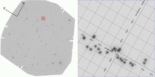
Left: the region surrounding Luhman 16 AB, as monitored by HST. It has dimensions of about 160″ × 160″ and is the sum of the stacks in WFC3/UVIS/F814W obtained for each of the 12 individual visits considered in this work. Right: zoom-in of the same image in the portion highlighted by a red square. It has a size of 7″ × 7″ and shows the complete pattern in the sky of Luhman 16 A and B during the period monitored by our HST observations. The orientation is the one of the master frame, while a fine grid (1″) gives equatorial coordinates.
In the next two sections, we will describe the determination of the astrometric and orbital parameters of the Luh 16 AB system employing two different methods.
4 METHOD A: SIMULTANEOUS DETERMINATION OF ASTROMETRIC AND ORBITAL PARAMETERS
Our reference system is not an absolute reference frame, as even the stars that moved the least and with the most robust positions are not at an infinite distance. On the basis of a Besançon Galactic model (Robin et al. 2004), we expect that our best measured stars used to define the (X, Y) reference frame lie at an average distance of ∼5 kpc. This would introduce a correction from relative to absolute of about 0.2 mas to our parallax and motions.
As noted previously, in this first analysis we aim for an accuracy equivalent to geometric distortion, about 0.3 mas. Hence, to first approximation, we assume our measured positions are on an absolute system. Rather than fitting the relative orbit (seven parameters) and the absolute motion of the baricentre plus the mass ratio (six parameters) separately, a 13-parameter model of the independent motions of Luhman 16 A and B is adopted. In terms of complexity, the computational cost of fitting both models is the same; however, fitting a model looking at the separate component motions makes it possible to measure the correlation between any pair of the 13 parameters, and thus deviation from that model for a planet orbiting one of the components.
In these nested minimizations, the inner one is linear and thus takes no iteration to reach the minimum. Therefore, one ends up with a simpler non-linear model with four parameters only. An initial guess of that four-dimensional non-linear problem can be obtained through a basic grid search before the whole 13-parameter non-linear objective function is minimized with, say, Levenberg–Marquardt.
The residuals of this model exhibit a seasonal variation along both axes (α* and δ) for both components. The periodicity (one year) and the fact that this variation is present in every residual rule out the presence of a companion as an explanation. If, instead of these natural residuals versus time, one plots the residuals in X and Y versus xraw and yraw, the seasonal variation becomes a straight line, thus revealing the presence of some CTE residual in the observations. Four straight lines are adjusted to correct for CTE: one for each axis and each filter. [Note that at each of the 13 epochs we have three observations in two coordinates, so 72 independent data points, for 12 epochs.] Once the CTE residuals are corrected for, a new model fit is carried out. The 13 parameters resulting from that minimization are listed in Table 4. The typical residual is 0.39 mas.
Astrometric and orbital parameters of Luhman 16 AB obtained with a simultaneous fit described in Section 4. The coordinates are in J2000.0, epoch 2015.0.
| α* (°)a | +96.9342078 | ±7.68E−07 |
| δ (°) | −53.3179180 | ±5.06E−07 |
| ϖ (mas) | 501.14 | ±0.052 |
| |$\mu _{\alpha ^*}$| (mas yr−1) | −2763 | ±1.45 |
| μδ (mas yr−1) | +358 | ±1.75 |
| A (mas) | +530 | ±58.8 |
| B (mas) | −410 | ±348 |
| F (mas) | +49 | ±1490 |
| G (mas) | −183 | ± 1250 |
| e | 0.25 | ±0.0648 |
| P (yr) | 19 | ±20.2 |
| T0 (Julian yr) | 2000 | ±24.6 |
| ρ | +1.22 | ±0.0214 |
Note.aα* = α cos δ.
Despite the exquisite precision of the HST data, there are difficulties in obtaining a reliable simultaneous fit of the astrometric and orbital parameters using only a partial arc of the orbit. It is particularly unsatisfactory that the orbital period that results is largely unconstrained (see Table 4), and so too the individual masses. Similar difficulties to obtain a simultaneous fit were reported previously by Sahlmann & Lazorenko (2015, section 3.1), who used an even shorter orbital arc than ours. Among other inconsistencies in their simultaneous solutions, they noted a strong anticorrelation between the residuals for the A and B components much larger than their measurement uncertainties, indicating that the motion of A and B were not independent and should be modelled globally. We therefore analysed our own A and B motion residuals, and found that the Pearson correlation coefficients are ∼0.65 for both the α* and δ components of our solution, indeed indicating a degree of correlation much larger than our expected uncertainties.
It is not clear how and why the accuracy of the simultaneous fit solution is degraded using a partial arc of the orbit. We suspect a complicated interplay with CTE residuals, field-targets colour dependencies in the PSFs, or just the deviations from the absolutes positions, all of which might propagate in the solution.
Therefore, until distances with Gaia for the reference field stars or data covering more of the orbital phase will be available, we now abandon the simultaneous fit of (absolute) astrometric and orbital parameters, and explore in the next section a simpler and more robust (relative) approach.
5 METHOD B: TWO-STEP DETERMINATION OF ASTROMETRIC AND ORBITAL PARAMETERS
In a two-body system, at any time, the baricentre (indicated hereafter with G) lies along the segment connecting the two components of the system, and the position of G along this segment is fixed by just one parameter, the mass ratio (hereafter, q).
In this second approach, we obtain our solution in two steps. In the first step, we determine q and the astrometric parameters of G (positions, proper motions, and parallax), and in the second step, we solve for the relative orbit, now using just the Luh16 A and B relative positions. Note that the derived astrometric parameters will be in the relative astrometric system of the reference frame (2X, 2Y), which is not an absolute system. The orbital solutions will not be affected by CTE residuals, because when looking at differences between A and B positions the effects of CTE should cancel out at a great level of accuracy. The same is true for the PSFs' colour dependencies, as Luh 16 A and B have essentially the same colour and they would be affected by the same systematic errors.
5.1 Step 1: determination of positions, parallax, proper motions, and mass ratio
In Fig. 1, we can see in one shot all the projected space motions during the first 12 epochs of our HST campaign in the period between 2014 August 22 and 2016 October 4, for both Luhman 16 A and B. Not all of the components in all the epochs are clearly distinguishable in this stacked image. More clear is Fig. 2, where we show the complete series of observed positions on the same reference frame (2X, 2Y) of Fig. 1, indicating Luhman 16 A with a filled dot, and B with an open circle. To better identify the epoch pair, we connect the AB components with a black segment. Note that at each given epoch (i.e. one single-orbit HST visit), there are actually three dithered individual observations taken less than an hour apart, which we can safely consider collected at the same astrometric epoch.
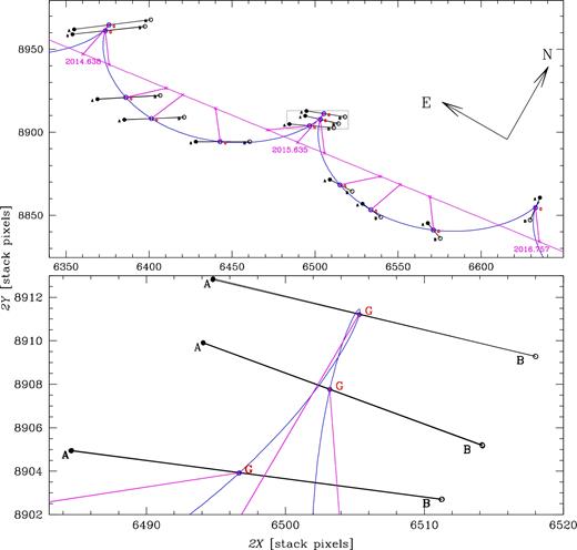
The top panel shows the complete series of observed positions for Luhman 16 A (filled circles) and Luhman 16 B (empty circles) in the coordinate system of our master frame. At any given epoch, a black line join A and B, and along it is marked with a red cross the position of the baricentre, G, estimated as explained in the text. A blue curve indicate the astrometric solution for the Luhman 16 AB's baricentre (positions, proper motions, and parallax), noting that the mass ratio, q, (i.e. the baricentre itself) is part of the solution. A line in magenta indicates the same solution with the system at an infinite distance, and crosses in magenta on this line indicate the individual epochs on this. These locations are connected with the observed baricentric positions. The orientations in this plot are the same of the master frame, as in Fig. 1. The bottom panel shows details for these curves around epoch 2015.6, in a region indicated in the top panel with a grey rectangle; this panel shows how finely observations were reproduced.
From the observed 36 2D data points, we would like to derive for the baricentre of the Luhman 16 AB system (G) five astrometric parameters: its positions (XG, YG), its motions |$(\mu _{X_{\rm G}},\mu _{Y_{\rm G}})$|, and most importantly, the system parallax π. However, the baricentre G is not an observable, but needs to be inferred from the relative positions of A and B components along their mutual orbit. So, we need to add to the unknown parameters the mass ratio q defined as |$\mathcal {M}_{\rm B}/\mathcal {M}_{\rm A}$| (i.e. 0 < q < 1, where |$\mathcal {M}$| indicate the mass of each component). In the following, we will describe the procedure followed to fit these six parameters.
By virtue of the principle that any transformation of the observational data degrades them, while numerical models do not, we perform this numerical fitting process directly in the observational plane (2X, 2Y). To accomplish our fit, we proceed iteratively solving for the best fit of the data, then de-trending for CTE residuals, and finally fitting again the CTE-de-trended data.
To predict the position of the baricentre, we make use of the sophisticated tool by U.S. Naval Observatory, the Naval Observatory Vector Astrometry Software, hereafter novas5 (in version F3.1, Kaplan et al. 2011), which accounts for many subtle effects, such as the accurate Earth orbit, perturbations of major bodies, nutation of the Moon–Earth system, etc. We are not interested in the absolute astrometric calculations of novas but only in the relative effects. In computing the positions we used an auxiliary star with no motion and zero parallax (i.e. at infinite distance), and finally compute the difference with respect to our targets. We then use a Levenberg–Marquardt algorithm (the fortran version lmdif available under minipack, Moré, Garbow & Hillstrom 1980) to find the minimization of six parameters: |$X_{\rm G},Y_{\rm G},\mu _{X_{\rm G}},\mu _{Y_{\rm G}},\pi$|, and q.
The first iteration produced a solution with residuals as large as 2 mas, which were significantly larger than our expected errors, and most importantly clearly and simply correlated with the xraw and yraw coordinates. We ascribed these residual mainly to CTE, but potentially also to differential chromatic and PSFs residuals correlated with roll angles. The best fit is shown with a blue line in Fig. 2. A simple fit to the residuals of the observed−calculated (O−C) of baricentre 2X and 2Y as function of xraw and yraw deliver a correction that can be applied to the (X, Y) positions. We refer to these de-trended positions for both A and B components with the symbols (Xdtr, Ydtr), which are given in Table 5. After this correction, the (O−C) residuals are perfectly consistent with those expected for stars of this luminosity for WFC3/UVIS, i.e. 0.008 pixels, or, 320 μmas. Therefore, we impute these remaining residuals to just random errors.
De-trended coordinates for Luhman 16 A and B, with magnitudes and quality fit parameter.
| Number ID | |$X_{\rm A}^{\rm dtr}$| | |$Y_{\rm A}^{\rm dtr}$| | QA | magA | |$X_{\rm B}^{\rm dtr}$| | |$Y_{\rm B}^{\rm dtr}$| | QB | magB |
|---|---|---|---|---|---|---|---|---|
| 01 | 3177.4290 | 4480.9726 | 0.0595 | −13.7789 | 3200.5478 | 4483.9043 | 0.0678 | −13.7686 |
| 02 | 3177.4385 | 4480.9813 | 0.0554 | −13.7958 | 3200.5502 | 4483.9105 | 0.0712 | −13.7514 |
| 03 | 3176.9600 | 4479.4869 | 0.0706 | −13.7721 | 3198.7869 | 4481.8681 | 0.0822 | −13.7836 |
| 04 | 3176.9733 | 4479.4917 | 0.0642 | −13.7539 | 3198.7938 | 4481.8611 | 0.0747 | −13.7483 |
| 05 | 3184.4585 | 4459.9941 | 0.0569 | −13.7644 | 3203.3598 | 4461.1151 | 0.0758 | −13.7225 |
| 06 | 3184.4847 | 4459.9796 | 0.0662 | −13.7687 | 3203.3837 | 4461.0890 | 0.0822 | −13.5614 |
| 07 | 3192.5618 | 4453.7872 | 0.0606 | −13.7936 | 3210.5695 | 4454.5485 | 0.0789 | −13.7416 |
| 08 | 3192.5604 | 4453.7906 | 0.0657 | −13.7925 | 3210.5842 | 4454.5426 | 0.0714 | −13.7596 |
| 09 | 3214.0726 | 4447.1540 | 0.0486 | −13.7717 | 3230.2991 | 4447.1838 | 0.0573 | −13.8035 |
| 10 | 3214.0726 | 4447.1658 | 0.0520 | −13.7789 | 3230.3068 | 4447.2018 | 0.0745 | −13.7369 |
| 11 | 3242.2729 | 4452.4620 | 0.0560 | −13.7351 | 3255.6101 | 4451.3406 | 0.0756 | −13.7226 |
| 12 | 3242.3008 | 4452.4571 | 0.0636 | −13.7869 | 3255.6356 | 4451.3474 | 0.0668 | −13.7521 |
| 13 | 3247.3892 | 4456.3960 | 0.0562 | −13.7746 | 3259.0011 | 4454.6361 | 0.0623 | −13.7179 |
| 14 | 3247.3943 | 4456.4028 | 0.0615 | −13.7785 | 3259.0115 | 4454.6309 | 0.0709 | −13.7319 |
| 15 | 3247.0500 | 4454.9440 | 0.0645 | −13.7750 | 3257.0941 | 4452.5905 | 0.0723 | −13.8075 |
| 16 | 3247.0505 | 4454.9441 | 0.0696 | −13.7775 | 3257.0982 | 4452.5800 | 0.0804 | −13.7487 |
| 17 | 3254.4639 | 4435.7605 | 0.0700 | −13.7896 | 3261.1670 | 4432.2108 | 0.0666 | −13.7592 |
| 18 | 3254.4500 | 4435.7624 | 0.0735 | −13.7754 | 3261.1665 | 4432.2065 | 0.0804 | −13.7109 |
| 19 | 3264.2620 | 4428.4694 | 0.0685 | −13.8066 | 3269.8034 | 4424.4836 | 0.0635 | −13.8043 |
| 20 | 3264.2910 | 4428.4512 | 0.0777 | −13.7803 | 3269.8294 | 4424.4669 | 0.0838 | −13.7612 |
| 21 | 3283.9466 | 4422.6495 | 0.0872 | −13.8059 | 3287.6769 | 4418.0644 | 0.0925 | −13.7280 |
| 22 | 3283.9666 | 4422.6405 | 0.0800 | −13.8129 | 3287.6971 | 4418.0447 | 0.0858 | −13.7983 |
| 23 | 3317.7075 | 4430.3043 | 0.0729 | −13.8042 | 3314.7639 | 4423.5710 | 0.0730 | −13.7451 |
| 24 | 3317.7254 | 4430.3247 | 0.0736 | −13.7757 | 3314.7844 | 4423.5749 | 0.0851 | −13.7410 |
| 25 | 3177.4511 | 4480.9871 | 0.0438 | −12.5274 | 3200.5524 | 4483.9125 | 0.0326 | −11.8824 |
| 26 | 3176.9679 | 4479.5222 | 0.0549 | −12.4756 | 3198.7734 | 4481.8883 | 0.0542 | −11.8233 |
| 27 | 3184.4647 | 4459.9898 | 0.0608 | −12.5185 | 3203.3521 | 4461.1134 | 0.0353 | −11.8406 |
| 28 | 3192.5469 | 4453.8118 | 0.0426 | −12.5346 | 3210.5591 | 4454.5391 | 0.0418 | −11.8384 |
| 29 | 3214.0780 | 4447.1755 | 0.0514 | −12.5449 | 3230.3074 | 4447.1921 | 0.0474 | −11.8699 |
| 30 | 3242.3070 | 4452.4713 | 0.0514 | −12.4980 | 3255.6328 | 4451.3491 | 0.0495 | −11.8312 |
| 31 | 3247.4004 | 4456.4198 | 0.0377 | −12.5136 | 3259.0075 | 4454.6286 | 0.0336 | −11.7717 |
| 32 | 3247.0462 | 4454.9560 | 0.0514 | −12.5031 | 3257.0802 | 4452.6036 | 0.0472 | −11.8295 |
| 33 | 3254.4352 | 4435.8009 | 0.0692 | −12.5472 | 3261.1611 | 4432.2221 | 0.0551 | −11.8479 |
| 34 | 3264.2919 | 4428.4862 | 0.0422 | −12.5278 | 3269.8101 | 4424.4895 | 0.0492 | −11.8609 |
| 35 | 3283.9286 | 4422.6551 | 0.0405 | −12.5847 | 3287.6626 | 4418.0566 | 0.0542 | −11.8742 |
| 36 | 3317.7059 | 4430.3364 | 0.0445 | −12.4950 | 3314.7809 | 4423.6060 | 0.0438 | −11.8031 |
Our final astrometric solution is given in Table 6. To assess uncertainties, we conservatively used the method of residual permutation, and take the 68th percentile of the deviations from the mean as the 1σ error. The relative parallax (which we indicate with π) is with respect to the most distant objects in the field (i.e. those that moved the least) and therefore π is only a lower limit to the absolute parallax ϖ. In a first approximation, we can use the relative-to-absolute correction, which was derived by SL15 as 0.28 ± 0.01 mas. In Table 6, we also give the value derived for ϖ employing this correction. However, we note that our relative parallax, π = 501.118 ± 0.093 mas, is already significantly larger than the absolute parallax by SL15, which is ϖ = 500.51 ± 0.11 mas, therefore implying a closer distance for Luh 16 AB, at no more than 1.9955 ± 0.0004 pc. When Gaia parallaxes for reference stars will become available we will be able to determine an accurate relative-to-absolute correction for our π value.
Astrometric parameters and mass ratio of Luhman 16 AB.
| q = |$\mathcal {M}_{\rm B}/\mathcal {M}_{\rm A}$| | 0.848 | ±0.023 |
| αJ2000.0 (h) | 10.82187776 | ±65 mas |
| δJ2000.0 (°) | −53.3193958 | ±45 mas |
| |$\mu _{\alpha \cos {\delta }_{\rm J2000.0}}$| (mas yr−1) | −2762.2 | ±2.3 |
| |$\mu _{\delta _{\rm J2000.0}}$| (mas yr−1) | 354.5 | ±2.8 |
| π (mas) | 501.118 | ±0.093 |
| ϖ = π + 0.28 ± 0.01 (mas) | 501.398 | ±0.093 ±0.01 |
5.2 Step 2: determination of the orbital parameters
With q and the astrometric parameters of G derived in the previous step, the position of the baricentre is known at any given epoch. This enables us to plot in Fig. 3, the observed data points in equatorial coordinates relative to the baricentre, revealing that our data cover over 120° of the projected true anomaly along the orbits (i.e. ∼1/3 of the projected orbit). We indicate the area swept during our observations with grey regions for both A and B components. For reference, we also show the A-B mass-reduced orbits for the solution derived later in this section. The relative positions, in equatorial coordinates, of Luhman 16 B with respect to Luhman 16 A are shown in Fig. 4 and given in Table 7.
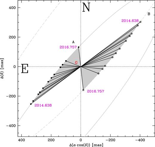
In equatorial coordinates, the positions of A and B components of Luhman 16 relative to our estimate of their common baricentre (indicated with G). We have also indicated the arc of the two baricentric orbits (solid line for A, and dashed line for B) and shaded the orbital area mapped during this HST campaign. Note the over 120° covered by the projection of the true anomaly.
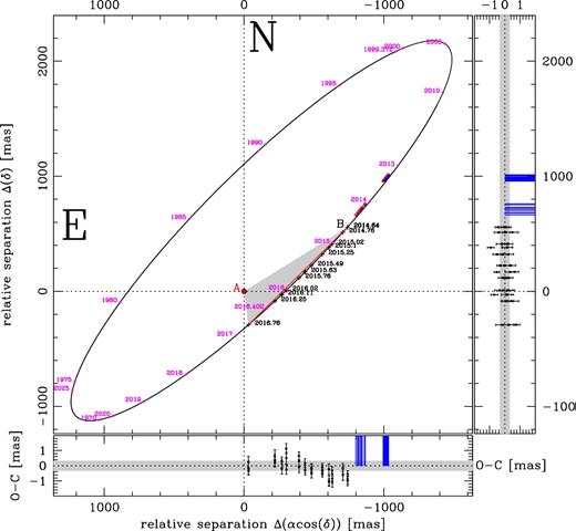
The relative orbit of Luhman 16 B around A. To better highlight the amount of curvature observed with HST (+symbols) in the A-B relative orbit, a red line connects the last with the first of the observed relative positions for the B component. The lower and right panels show in mas the (O−C) residuals with respect to our best orbital model. A grey band is given for reference as the expected uncertainty for any individual positional measurement (0.32 mas). Red circles show the positions available from the Sahlmann & Lazorenko (2015), they are all out of scale in the O−C panels. Blue lines connect the individual SL15 data points with their expected positions on our orbital solution at the epoch those observations were collected. See Fig. 5 for a more meaningful comparison of residuals.
Cartesian relative equatorial positions of B with respect to A with estimated errors, in mas.
| Number ID | Julian Year | Δα cos δ | Δδ | σΔ |
|---|---|---|---|---|
| (mas) | (mas) | (mas) | ||
| 01 | 2014.63801 | −740.243 | 557.536 | 0.319 |
| 02 | 2014.63820 | −740.047 | 557.310 | 0.319 |
| 03 | 2014.75865 | −706.509 | 513.032 | 0.383 |
| 04 | 2014.75873 | −706.521 | 512.498 | 0.348 |
| 05 | 2015.02328 | −630.386 | 411.781 | 0.335 |
| 06 | 2015.02347 | −630.535 | 411.335 | 0.373 |
| 07 | 2015.10044 | −606.637 | 381.725 | 0.352 |
| 08 | 2015.10053 | −607.376 | 381.722 | 0.343 |
| 09 | 2015.25312 | −559.585 | 321.314 | 0.266 |
| 10 | 2015.25321 | −559.728 | 321.680 | 0.321 |
| 11 | 2015.49489 | −482.563 | 224.543 | 0.333 |
| 12 | 2015.49507 | −482.249 | 224.899 | 0.326 |
| 13 | 2015.63458 | −435.605 | 168.446 | 0.297 |
| 14 | 2015.63467 | −436.025 | 168.136 | 0.332 |
| 15 | 2015.75923 | −393.198 | 117.008 | 0.342 |
| 16 | 2015.75932 | −393.531 | 116.713 | 0.376 |
| 17 | 2016.01960 | −301.470 | 9.767 | 0.342 |
| 18 | 2016.01969 | −302.055 | 9.818 | 0.385 |
| 19 | 2016.11147 | −269.974 | −28.218 | 0.330 |
| 20 | 2016.11167 | −269.841 | −28.225 | 0.404 |
| 21 | 2016.24932 | −219.280 | −84.655 | 0.449 |
| 22 | 2016.24948 | −219.498 | −85.021 | 0.415 |
| 23 | 2016.75726 | −31.285 | −290.547 | 0.365 |
| 24 | 2016.75735 | −31.701 | −291.065 | 0.398 |
| 25 | 2014.63805 | −739.763 | 556.973 | 0.193 |
| 26 | 2014.75869 | −706.069 | 512.088 | 0.273 |
| 27 | 2015.02332 | −629.855 | 411.596 | 0.249 |
| 28 | 2015.10048 | −607.463 | 380.640 | 0.211 |
| 29 | 2015.25316 | −559.945 | 320.916 | 0.247 |
| 30 | 2015.49494 | −482.185 | 224.290 | 0.252 |
| 31 | 2015.63462 | −436.057 | 167.271 | 0.179 |
| 32 | 2015.75927 | −392.827 | 116.847 | 0.247 |
| 33 | 2016.01964 | −302.832 | 9.213 | 0.313 |
| 34 | 2016.11159 | −269.388 | −29.052 | 0.229 |
| 35 | 2016.24936 | −219.672 | −85.045 | 0.239 |
| 36 | 2016.75731 | −31.870 | −290.080 | 0.221 |
To determine the seven orbital parameters of visual binaries, we will follow the trial-and-error approach described by Pourbaix (1994). We employed the two software tools developed and maintained by one of us (DP): union and epilogue (Pourbaix 1998a). Practical details about the internal algorithms and some applications are available in Pourbaix (1998a,b; 2000). Briefly, union and epilogue are used together to simultaneously adjust the observations of double-lined spectroscopic-visual binaries (VB-SB2). union undertakes a global optimization then followed by a preliminary local search. In order to increase the chance of getting the right minimum, the user supplies with a time range to which the orbital period is assumed to belong. epilogue processes the results of union and generates some statistical information as well as ephemerid for the solution.
The resulting orbital solution for the Luhman 16 A-B system is given in Table 8. To estimate uncertainties, we use the conservative approach of permuting the 36 residuals. We give the minimum and maximum values of the different realizations, and their weighted averages. We indicate in the case of ω and Ω that a 5σ clipping exclude four outliers.
Derived orbital parameters and masses of Luh 16 AB.
| Parameter | Min value | Max value | Weighted mean ± σ |
|---|---|---|---|
| a (″) | 1.69 | 2.84 | 1.91 ± 0.25 |
| a (au) | 3.71 | 5.67 | 3.81 ± 0.50 |
| i (deg) | 78.51 | 80.10 | 79.21 ± 0.45 |
| ω (deg) | 84 | 168a(307) | 107a ± 18 |
| Ω (deg) | 127.6 | 132.2a(311) | 130.3a ± 1.1 |
| e | 0.31 | 0.61 | 0.46 ± 0.06 |
| P (yr) | 24.5 | 64.4 | 31.3 ± 7.9 |
| T° (Julian yr) | 2016.2 | 2018.4 | 2017.1 ± 0.7 |
| |$\mathcal {M}_{\rm tot}^b$| (|$\mathcal {M}_{{\odot }}$|) | 0.044 | 0.085 | 0.056 ± 0.020 |
| |$\mathcal {M}_{\rm tot}^b$| (|$\mathcal {M}_{\rm J}$|) | 46 | 89 | 59 ± 21 |
| |$\mathcal {M}_{\rm Luh\,A}^c$| (|$\mathcal {M}_{\rm J}$|) | 26 | 48 | 32 ± 11 |
| |$\mathcal {M}_{\rm Luh\,B}^c$| (|$\mathcal {M}_{\rm J}$|) | 21 | 41 | 27 ± 10 |
Notes.a5σ clipped, rejecting four outliers.
Total mass, b|$\mathcal {M}_{\rm tot} = \mathcal {M}_{\rm Luh\,16\,A} + \mathcal {M}_{\rm Luh\,16\,B} = a^3/P^2$|.
cAssuming q = 0.848, |$\mathcal {M}_{\rm Luh\,16\,A} = 1/(1+q) \mathcal {M}_{\rm tot}$|, and |$\mathcal {M}_{\rm Luh\,16\,B} = q/(1+q) \mathcal {M}_{\rm tot}$|.
5.3 Disagreement with SL15 astrometry
We have downloaded the online Supporting Information available at MNRAS, for table A1 of the Sahlmann & Lazorenko (2015) study.6
This table provides the equatorial coordinates of Luhman 16 A and B collected with FORS2@VLT in 22 epochs between 2013 April 14 and 2014 May 18. The positions are given in the ICRS, after a correction for differential colour refraction (DCR) effects was applied.
These data points could potentially extend by 1.36 yr our HST data time base-line, resulting in better estimates of both astrometric and orbital parameters. Extra monitoring would also improve the search for perturbations induced by third bodies.
We show the relative positions transformed into the tangential plane in Figs 4 and 5 as small red circles. Apparently the SL15 data points are not consistent with our orbital solution. We attempt to re-derive the orbital fit including also SL15 data but with no success. No simple rotation nor shift can solve the inconsistency. However, if we assume the pixel scale in SL15 to be off by ∼5 per cent, the data would be nearly aligned with our orbital solution. But, even when this is assumed, and the orbit is re-derived using our HST data points and simultaneously including SL15 data points, the results are not physically consistent. In summary, we are unable to fit simultaneously our HST data and those by SL15 collected at FORS2@VLT.
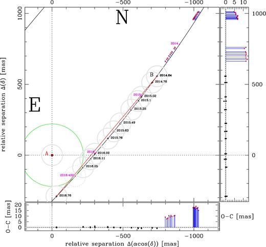
Same as in Fig. 4, only focused on the observed data points from this work and from SL15. The residuals are now shown in a scale that enable to see all residuals of the SL15 data points. Note that neither a simple rotation or shifts, nor a change in the absolute scale can bring into agreement SL15's VLT data points with our HST's data set. A green circle indicates the apparent periastron (at 220.5 mas) estimated to have happened in 2016.402. For reference, the size of the nominal full width at half-maximum with WFC3/UVIS filter F814W (74 mas) is indicated with a grey thick circle at positions where A and B components were observed, and dotted at the not-observed apparent periastron.
In Fig. 5, it can be appreciated that while our observed HST data points significantly deviate from the straight line (by over 25 mas, at ∼100σ) those observed by SL15 are almost consistent with a straight line, deviating no more than very few mas, which seems consistent with the observed amount of scatter in their 22 data points. This is also consistent with the fact that while our HST data are exploring over 120° of the projected true anomaly ν, the SL15 data map only a few degrees of ν (see Fig. 4). This is even clearer in Fig. 6, where the amount of curvature traced by our HST data is better exposed.
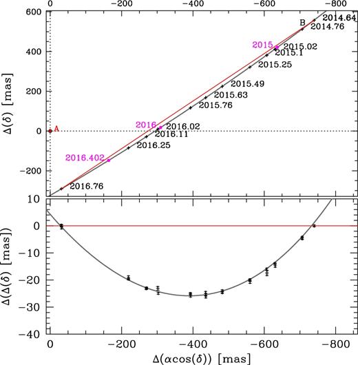
We cannot point to the exact reason(s) of these discrepancies, however, we suspect the usual limitations of ground-based facilities may be responsible, i.e.: (i) the limited parallax factor covered by the ground-based data (see fig. 3 of SL15); (ii) the FORS2 geometric astrometric stability (camera focal enhancing, de-rotator, and active optic stability) and the effects of Earth's atmosphere on the astrometry (variable PSFs, variable extinction, and residual DCR); (iii) the limited angular resolution for this tight binary (∼1″ during 2013–2014, i.e. comparable to the ground-based seeing); and (iv) the limited arc of the AB orbit the ground-based data cover. SL15 quote positional errors within individual images as low as 0.25 mas, and we suspect that this quoted uncertainty – below the HST geometric distortion limit – reflects only internal errors, which might severely underestimate the true (internal and systematic) errors. Nevertheless, their orbital solution, although poorly constrained by the data, still gives (O−C) residuals consistent with their quoted errors. It is also unclear whether in deriving their proper motions they made use of the original WISE AB-photocentre position (of the unresolved components). Instead, we are only using our 2014–2016 HST data, as using unresolved position of the photocentre (and at a different wavelength) would surely result in decreasing the accuracy of our solution, biasing our estimates for astrometric parameters of G and q.
6 COMPARISON WITH RADIAL VELOCITIES FROM THE LITERATURE
In deriving the orbit of a visual binary from astrometry only, the inclination (which appears as cos i) is degenerate in i and −i and only RVs can remove this degeneracy and determine the sign. Thankfully, a couple of RVs measurements are available from the literature and epilogue and union can process RVs (Pourbaix 1998a).
The only suitable resolved heliocentric RVs available from the literature are the ones of Kniazev et al. (2013) and Crossfield et al. (2014). Kniazev et al. at epoch 2013.196 give 23.1 ± 1.1 and 19.5 ± 1.2 km s−1, for components A and B, respectively. Crossfield al. at epoch 2013.342 give for 20.1 ± 0.5 and 17.4 ± 0.5 km s−1, for components A and B, respectively.
Inevitably, there are numerous difficulties to estimate the absolute RV zero-points of heterogeneous observations collected with different instruments at different telescopes in different sites, and this is particularly true when comparing RVs derived from optical and IR observations. Therefore, as we are interested mainly in the relative RVs of the two components, we assumed the mass ratio q derived in Section 5.1, and compute the RVs of the baricentre for the two references. We then impose the velocity of the baricentre in the two data sets to be equal. This was obtained imposing a shift of +2.6 km s−1 to the Crossfield et al. data.
In Fig. 7, we compare our orbital solution with our astrometric data points and with the available RVs processed as just described above. From top to bottom, we show our residuals as function of δ, α*, and RVs. These two RV pairs are sufficient to suggest that i should have a negative value. Consequently, also the ω and Ω change by 180°. For clarity, the new amended values are given in Table 9.
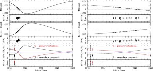
From top to bottom, the three panels show the comparisons between the observed Δ(δ), Δ(α cos δ), RVs, and the corresponding quantities from our best orbital fit for the Luhman 16 AB system. Each comparison also shows the observed−calculated values below the corresponding panels. The RVs available from literature were processed as described in the text. Left: we show the models over a full A-B orbital period as reference for the expected full amplitudes of these quantities, although observations are currently limited to just ∼3.5 yr. Right: same plot, but focused just on the time interval where data are actually available so far.
Final orbital parameters and masses of Luhman 16 AB.
| a (″) | 1.91 | ±0.25 |
| a [au] | 3.81 | ±0.50 |
| i [deg] | −79.21 | ±0.45 |
| ω [deg] | 287 | ±18 |
| Ω [deg] | 310.3 | ±1.1 |
| e | 0.463 | ±0.064 |
| P [yr] | 31.3 | ±7.9 |
| T0 [Julian yr] | 2017.12 | ±0.65 |
| |$\mathcal {M}_{\rm tot}$| [|$\mathcal {M}_{{\odot }}$|] | 0.056 | ±0.020 |
| |$\mathcal {M}_{\rm tot}$| [|$\mathcal {M}_{\rm J}$|] | 59 | ±21 |
| |$\mathcal {M}_{\rm Luh\,A}$| [|$\mathcal {M}_{\rm J}$|] | 32 | ±11 |
| |$\mathcal {M}_{\rm Luh\,B}$| [|$\mathcal {M}_{\rm J}$|] | 27 | ±10 |
7 PHOTOMETRY
Our HST photometry were calibrated to the Vega magnitude system by adding the filter zero-points (ZP|$_{m_{\rm F814W}} = 29.02\pm 0.02$| and ZP|$_{m_{\rm F606W}} = 32.24\pm 0.02$|, following Bedin et al. 2005)7 to the instrumental magnitudes given in Table 5. The absolute accuracy of the calibration is about 0.02 mag per filter. Our observations are not well suited for constraining rotational modulation of these sources, but provide some of the most precise optical photometry for the two BDs.
In Fig. 8, we summarize the photometry obtained for the targets (Luh 16 A in blue, and B in red) and for the sources in our WFC3/UVIS field (black square symbols). On the left-hand panel, we show the (mF606W − mF814W) versus mF814W colour–magnitude diagram (CMD). The onset of saturation in the 60 s exposure in F814W is indicated by a dotted line. Note how Luh 16 A and B are considerably redder than any other source in the field, and just below the saturation level (as planned). On the right-hand panels, we show our registered and calibrated magnitudes obtained for each image. The error bars associated with each data points is the rms for stars within 1 mag below the saturation level. This is 0.01 for all, with the exception of B in F606W, for which we associate an error of 0.0125 mag. Both Luh 16 components appear to have a scatter considerably larger than field objects of the same magnitudes, in particular the B component.
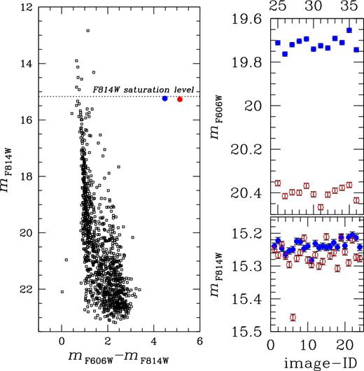
Summary of the photometric data released as part of this work. Black symbols are field objects observed within our WFC3/UVIS field, Luh 16 A is indicated in blue and Luh 16 B in red. On the left-hand panel, we show the CMD of all the sources. A dotted line indicate the onset of saturation. On the right-hand panels, we show the individual magnitudes for Luh 16 A and B (F606W on top, and F814W on bottom), as measured in each of the 36 images used in this work, as function of the image number ID (Table 1).
Luhman 16 B is one of the highest amplitude variable BD known (Biller et al. 2013; Gillon et al. 2013; Buenzli et al. 2014, 2015a) and spatially resolved studies discovered variability also in Luhman 16 A (Buenzli et al. 2015a) emerging from the rotation of the heterogeneous cloud deck of the BD. Time-resolved precision photometry by Gillon et al. (2013) showed rapidly evolving light-curve variations in Luhman 16 B and multiband photometry and resolved ground-based spectroscopy by Biller et al. (2013) and Burgasser et al. (2013), respectively, showed wavelength- (and therefore pressure-) dependent phase shifts and amplitude variations. Buenzli et al. (2014, 2015a) used high-precision time-resolved HST spectroscopy (0.8–1.7 μm range) to show that correlated temperature and cloud thickness variations are responsible for the observed near-infrared (NIR) spectral evolution, similar to other variable L/T transition BDs (e.g. Radigan et al. 2012; Apai et al. 2013). Crossfield et al. (2014) presented time-resolved CO line profile observations to derive the first Doppler-imaging map for a BD, which revealed multiple bright and dark patches; Karalidi et al. (2015) used a Markov Chain Monte Carlo optimized forward modelling procedure (Aeolus, with a finely pixelized sphere and assuming elliptical structures) to derive the simplest surface brightness map that is consistent with the observed variations. Although taken hundreds of rotations apart and with different techniques, the Crossfield et al. and Karalidi et al. maps show some similarity in terms of the approximate size, distribution, and contrasts of the features.
The observed variability for component A is 0.11 mag in F606W and 0.08 mag in F814W, while for component B, we observed variations as large as 0.11 mag in F606W and 0.25 mag in F814W. These are significantly larger than the ∼0.01 photometric precision of our measurements. As our observations are not resolved on the time-scale of the rotational periods of Luhman 16 A and B, we cannot derive peak-to-peak changes for the objects, therefore the reported values should be considered lower limits on the intrinsic amplitudes at these wavelengths. Red-optical variability has been detected in other T dwarfs (e.g. Gillon et al. 2013; Heinze et al. 2015), which suggests that cloud amplitudes are likely as large if not larger in the red optical than they are in the NIR (1–1.6 μm) bands, potentially providing stronger constraints on condensate grain size distribution (e.g. Lew et al. 2016).
Alternately, variability of non-thermal emission induced by magnetic activity could be responsible for this signal, as such emission has a much greater relative impact at optical wavelengths where the photospheric emission is weak (e.g. Croll et al. 2016; Gizis et al. 2017). Magnetic emission has been detected from T dwarfs at optical (e.g. Burgasser et al. 2003; Kao et al. 2016; Pineda et al. 2016) and radio wavelengths (e.g. Route & Wolszczan 2012, 2016); however, neither component of Luhman 16 AB was found to exhibit Hα emission to an equivalent width limit of 1.5 Å (Faherty et al. 2014), and the system was undetected in single-epoch radio and X-ray observations (Osten et al. 2015). Further investigation into the variability of this system, over broad wavelength and time spans, is certainly warranted.
Our observations are also consistent with the extended baseline (spatially unresolved) photometric monitoring of the Luhman 16 AB system in the Pan-STARRS-Z band and in the Sloan Digital Sky Survey (SDSS) i΄ band, which show that modulations 0.05 mag are typical over the time-scales of the rotational period, but these authors also report changes as large as 0.1 mag (Street et al. 2015).
8 PRESENCE OF EXOPLANETS
The main goal of this project is to search for, and possibly to characterize, exoplanets and other bodies, in P-type or S-type orbits around the Luhman 16 A and B components. We summarize the results of this preliminary work as follow:
We inspected each epoch for faint companions, and find no detectable third-body comoving with the Luhman 16 A-B system within our WFC3/UVIS field of view. At 2 pc, our search area extends from 1 au (0|${^{\prime\prime}_{.}}$|5) to 80 au. Assuming a detection limit of mF814W=23 mag (Fig. 8), we can rule out well-resolved companions to an absolute magnitude limit of MF814W ≈ 26.5. For comparison, the T9 dwarf UGPS J072227.51−054031.2 has an absolute i-band magnitude of 26.2 (Leggett et al. 2012), so these observations rule out companions warmer than a Y dwarf (Teff ≳ 500 K). It appears that these new HST images do not provide any new constraints (from direct detection) that surpass those from Melso et al. (2015).
In Fig. 9, we show the amplitude of the expected astrometric perturbation for a number of cases, overimposed on our current 3σ threshold. For simplicity, we assume circular planetary orbits as these are more likely to be stable, and adopt the maximum and minimum masses for Luh 16 A and Luh 16 B, respectively, given in Table 8.
Using our HST-only data, we confirm the results by SL15 as we also do not see any significant residual in our motions at the ∼mas level compatible with the perturbation induced by a third body having a mass larger than 2 Jupiter Masses (|$\mathcal {M}_{\rm J}$|), and period between 20 and 300 d.
Our longer time baseline of 2.12 yr, compared to the SL15 baseline of 1.09 yr, allow us to exclude the presence of 2 |$\mathcal {M}_{\rm J}$| planets with period as long as 2 yr.
We can also exclude the presence of 1 |$\mathcal {M}_{\rm J}$| with period between 20 d and 2 yr.
Finally, we can extend this claim down to significantly lower masses, i.e. down to Neptune masses for periods longer than about 1 yr.
To increase sensitivity and place a lower limit to what we could detect, we can average the residuals before and after 2015.75, where there might seem to be a marginally significant residual of about 0.5 ± 0.2 mas (mainly in α*). Even assuming that this can be ascribed to a genuine signature caused by a third body – rather than a more likely effect of residual systematic errors – and assuming masses between the maximum and minimum masses for Luh A and B, it would imply a period larger than 2 yr and a mass not greater than one Neptunian mass.
Neither a simple shift, nor a rotation, nor a scale change can reconcile our HST-derived positions with those by SL15 based on data obtained with VLT from ground. The two data sets cannot be fit with a common orbital solution unless an ad hoc third body is used to explain that discontinuity; a possibility that at this stage we have not explored.
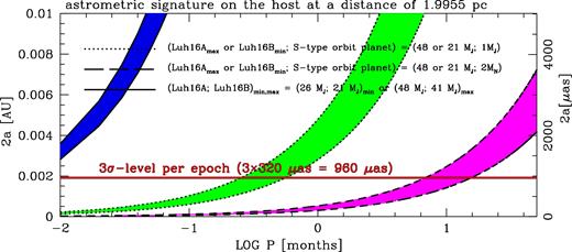
Assuming a distance of 1.9955 pc for Luhman 16 AB, and the maximum and minimum masses for Luh 16 A and Luh 16 B derived in Table 8, respectively, we show the relation between twice the semimajor axis 2a of the baricentric orbit of the luminous companions (A or B) around the centre of mass with a non-luminous planet, and the period (P). Dotted lines show this relation for a planet with a mass of 1 |$\mathcal {M}_{\rm Jupiter}$|. The green region indicates the loci for intermediate masses for A or B. The dashed lines (and corresponding region in magenta) indicate the corresponding astrometric signal induced by a 2 |$\mathcal {M}_{\rm Neptune}$| exoplanets. For reference, the solid lines (and blue region) show the amount of A-B orbital motion if the system was on a circular orbit. Twice the semimajor axes because that is the maximum size of the total range of motion for a circular orbit that we can measure. The horizontal red line sets our limit to the astrometric signal, i.e. 3σ ≃ 960 μas, or, for a distance of ∼2 pc, equivalent to ∼0.002 au (i.e. about 300 000 km).
9 ELECTRONIC MATERIAL
As part of this work, we electronically release as Supporting Information on the Journal: (i) The individual observed positions and magnitudes for A and B in the tables. (ii) The astrometrized stack of the HST observations in filter F814W. (iii) The photometry for the field objects.
10 CONCLUSIONS
In this paper, we presented the first results from an ongoing, high-precision, HST-based astrometric monitoring campaign targeting the Luhman 16 AB system, the closest BDs to the Sun. The key findings of our study are as follows:
We rule out comoving companions down to Y dwarf spectral types in the range 1–80 au. This result confirms the finding of Melso et al. (2015), which is based on superior data for this analysis. Note that Melso et al. also extended this investigation at wider separations.
Our HST data alone confirm the results by SL15: we find no evidence for ∼mas-level residuals that would be consistent with an exoplanet in the system with a mass greater than 2 |$\mathcal {M}_{\rm Jup}$| and with a period between 20 and 300 d.
We extend this results to lower masses and larger periods. In particular, no exoplanets with masses larger than a Neptunian mass and period between 1 and 2 yr.
Our measurements significantly improve the parallax and proper motion of the Luhman 16 AB system, and indicates that this system is closer to the Sun (<2 pc) than previous measurements.
We have also improved on the mass ratio q of the Luhman 16 AB system and mapped the motions through the apparent periastron.
Further significant improvements on the astrometric solution and parallax of the Luhman 16 AB system can be made in the near-future: we plan to focus on the trailed HST images already collected and those planned for 2018 August, to further improve the astrometric precision and search exoplanets down to few Earth masses. Follow-up observations with the VLT/CRIRES+ instrument will provide accurate RV data, an important complement to our 2D astrometric data, as it will provide the missed component necessary for the complete three-dimensional picture of the kinematic in the system. In addition, the Gaia DR2 data set will provide absolute motions, positions, and distances of several stars in the field, allowing us to link our positions to an absolute system.
Acknowledgments
We thank an anonymous referee for the critical and careful reading of our manuscript, and for her/his suggestions and corrections that have contributed to improve this work. DA and AB acknowledge support from STScI grants GO-13748 and GO-14330. We warmly thank Shelly Meyett and Peter McCullough at STScI, our Program Coordinator and Contact Scientist for their great support during the planning of the multiyear observations.
Based on observations with the NASA/ESA Hubble Space Telescope, obtained at the Space Telescope Science Institute, which is operated by AURA, Inc., under NASA contract NAS 5-26555, under GO-13748 and GO-14330.
WFC3 Instrument Handbook Chapter 2.2, Dressel (2017).
The Mikulski Archive for Space Telescopes (MAST) is a NASA funded project. MAST is located at the STScI. http://archive.stsci.edu/hst
REFERENCES
SUPPORTING INFORMATION
Supplementary data are available at MNRAS online.
sumF814W_gaiaWCS.fits.bz2
field.xyvi.bz2
Please note: Oxford University Press is not responsible for the content or functionality of any supporting materials supplied by the authors. Any queries (other than missing material) should be directed to the corresponding author for the article.
