


Abstract
Denmark has played a substantial role in the history of Northern Europe. Through a nationwide scientific outreach initiative, we collected genetic and anthropometrical data from ∼800 high school students and used them to elucidate the genetic makeup of the Danish population, as well as to assess polygenic predictions of phenotypic traits in adolescents. We observed remarkable homogeneity across different geographic regions, although we could still detect weak signals of genetic structure reflecting the history of the country. Denmark presented genomic affinity with primarily neighboring countries with overall resemblance of decreasing weight from Britain, Sweden, Norway, Germany, and France. A Polish admixture signal was detected in Zealand and Funen, and our date estimates coincided with historical evidence of Wend settlements in the south of Denmark. We also observed considerably diverse demographic histories among Scandinavian countries, with Denmark having the smallest current effective population size compared to Norway and Sweden. Finally, we found that polygenic prediction of self-reported adolescent height in the population was remarkably accurate (R2 = 0.639 ± 0.015). The high homogeneity of the Danish population could render population structure a lesser concern for the upcoming large-scale gene-mapping studies in the country.
DENMARK has played a substantial role in the history of Northern Europe. Like Swedes and Norwegians, Danes are historically linked to the Vikings—the Germanic Norse seafarers whose commercial and military operations marked the Viking Age in European history (793–1066). Through a series of invasions, conquests, and alliances, the Danish Vikings established settlements as far as in Britain, Estonia, the Faroe Islands, Iceland, Greenland, and even Canada. Denmark’s long-lasting historical bond with Sweden and Norway is nicely exemplified in the formation of the Kalmar Union, a state that brought together the three Scandinavian nations from 1397 to 1523 as a response to Germany’s expansionist tendency to the north (Derry 2000).
Denmark’s historical complexity is contrasted by the country’s small current size—both in terms of geographic area (∼43,000 km2) and population (5,614 million inhabitants)—a fact even further contrasted by the notable compartmentalization of the Danish linguistic map in ∼30 dialectal areas (http://dialekt.ku.dk/). These observations, together with the evident lack of strong geographic barriers in the country, make present-day Denmark an interesting setting for studying the genetic history of small populations with a glorious past.
In recent years, there has been an explosion of human genetic studies that contributed substantially to the characterization of worldwide variation patterns (Lao et al. 2008; Li et al. 2008; Novembre et al. 2008; Reich et al. 2009; Busby et al. 2015); the reconstruction of population history in regions with poor/nonexistent historical records (Moreno-Estrada et al. 2014; Moreno-Mayar et al. 2014); the study of local and global patterns of admixture in multiethnic societies (Bryc et al. 2015); and the study of admixture with other hominin species as well as its use in elucidating human dispersals (Green et al. 2010; Reich et al. 2011). The increased power of high-throughput genotype data and computational methods has also boosted the emergence of many single-country genomic projects in Europe (Jakkula et al. 2008; Price et al. 2009; Genome of the Netherlands Consortium 2014; Karakachoff et al. 2015; Leslie et al. 2015) and the release of useful data to the public (Welter et al. 2014).
In this work, we extend the collection of single-country genetic studies by introducing a new project from Denmark. Unlike previous genomic projects involving Denmark (Bae et al. 2013; Larsen et al. 2013), ours was conceived from the beginning as a scientific outreach initiative with benefits for both the general public and our research objectives. We invited high school students from across Denmark to participate in activities whose primary goal was to promote genomic literacy in secondary education (Athanasiadis et al. 2016). Most participants donated a DNA sample, which we used to explore the extent to which recent and more distant historical events left their mark on the genetic makeup of the Danish population. Apart from the population structure and demographic history in Denmark, an additional focus of this work has been the quantitative study of basic anthropometrical traits.
With this work, we ultimately report back to our DNA donors the biological and historical insights we gained from analyzing their genetic data. Our results showed remarkable homogeneity across different geographic regions in Denmark, although we were still able to detect weak signals of genetic structure. Denmark received substantial admixture contributions primarily from neighboring countries in the past 10 centuries with overall influence of decreasing weight from Britain, Sweden, and Norway. We also observed considerably diverse demographic histories among the Scandinavian countries, as reflected in their historical effective population size. Finally, we found that human height can be predicted with remarkable accuracy in Danish adolescents. Overall, this work showcases how far we can go with the analysis of genetic data from small, fairly homogeneous populations.
Materials and Methods
Sample description
New data:
We recruited ∼800 students from 36 high schools from across Denmark under the Where Are You From? project (Athanasiadis et al. 2016). These numbers correspond to the sampling of ∼1 in 9350 Danish inhabitants (Figure 1). We asked each participant to provide a saliva sample for DNA analysis and to answer an online questionnaire about family origin (their own, their parents’, and their grandparents’ place of birth) and basic anthropometrical data (e.g., self-reported height and weight). The institutional review board of Aarhus University approved the study. Because no health-related questions were asked, there was no requirement for additional approval by the university’s medical ethics committee. Informed consent was obtained either from the participants (age >18 years) or their parents (age <18 years). We used the 23andMe (Mountain View, CA) DNA analysis service for the genotyping of 723 participants. The 23andMe service uses a custom HumanOmniExpress-24 BeadChip from Illumina (San Diego, CA). After excluding duplicate single nucleotide polymorphisms (SNPs), applying a per-locus missingness threshold of 2% with PLINK v1.9 (Chang et al. 2015) and removing SNPs ambiguously mapped to the forward DNA strand, 517,403 unique autosomal SNPs were available for further analysis.
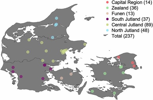
Location of the 36 Danish high schools participating in the Where Are You From? project colored by geographic origin. Number of samples with at least three grandparents born in each of the six regions is shown in parentheses.
Additional data:
To put our study in a broader European context, we included four additional data sets: (i) 2833 individuals × 227,899 SNPs from the Population Reference Sample (POPRES) (Nelson et al. 2008); (ii) 494 individuals × 314,526 SNPs from Amyotrophic Lateral Sclerosis (ALS) Finland (Laaksovirta et al. 2010); (iii) 381 individuals × 577,252 SNPs from the Swedish Schizophrenia Study (Ripke et al. 2013); and (iv) 300 individuals × 537,306 SNPs from the Norwegian Cognitive NeuroGenetics (NCNG) sample (Espeseth et al. 2012). We applied separate quality controls to these data sets according to their particularities (protocols available upon request).
Imputation
We carried out genotype imputation within each data set separately before combining them. We first changed DNA strand orientation of several SNPs in all five data sets to create a uniform forward orientation using SNPFLIP (https://github.com/endrebak/snp-flip) and PLINK. Supplemental Material, Table S1 shows the number of SNPs that were flipped/removed from each data set. We then used liftOver from the University of California Santa Cruz Genome Browser to “lift” genome coordinates from the National Center for Biotechnology Information (NCBI)36/hg18 (March 2006) to the GRCh37/hg19 (February 2009) assembly in the POPRES, ALS Finland, and NCNG data sets. We produced “prephased” haplotypes for each data set with SHAPEIT v2.720 (Delaneau et al. 2012) and used the haplotypes together with the latest 1000 Genomes Phase 3 reference panel (b37, October 2014) for the separate imputation of the five data sets with IMPUTE2 v.2.3.1 (Howie et al. 2012). Finally, we concatenated the imputed data into separate chromosomes and filtered them for “info” ≥0.975 with QCTOOL (http://www.well.ox.ac.uk/∼gav/qctool/#overview).
Principal component analysis
We ran principal component analysis (PCA) with PLINK to explore population structure in our Danish sample. PCA was run on two different data combinations: (i) POPRES, Where Are You From?, NCNG, and the Swedish Schizophrenia Study and (ii) Where Are You From?, NCNG, the Swedish Schizophrenia Study, and Germany from POPRES. To avoid undesirable clustering due to extensive linkage disequilibrium (LD), we thinned the genotypes with PLINK (using a window and step size of 1500 and 150 SNPs, respectively, and r2 threshold = 0.80) and removed SNPs from known high-LD genomic regions (e.g., MHC on chromosome 6).
Chromosome painting, population clustering, and admixture
We used a set of LD-based methods—CHROMOPAINTER (Lawson et al. 2012), fineSTRUCTURE (Lawson et al. 2012), and GLOBETROTTER (Hellenthal et al. 2014)—to explore fine-grain population structure and admixture in Denmark. These methods require a set of phased SNP data from “donor” (i.e., the available European samples) and “recipient” populations (i.e., the Danish sample). In brief, the methods detect extended multimarker haplotypes across the genome, which are organized in pairwise vectors of similarity counts (CHROMOPAINTER). These vectors are then used by an MCMC algorithm (fineSTRUCTURE) to hierarchically cluster individuals into groups that are often geographically, linguistically, and/or historically meaningful (Leslie et al. 2015). Admixture proportions are estimated through multiple linear regression on the average proportion of DNA that each recipient copies from each of the donor groups (GLOBETROTTER). Nonparametric standard errors of admixture proportions were calculated with a jackknife procedure described elsewhere (Montinaro et al. 2015). Finally, GLOBETROTTER also measures the decay of association vs. genetic distance between the “chromosome chunks” copied from a given pair of donor groups. This decay is exponentially distributed with rate equal to the time that the admixture occurred (Hellenthal et al. 2014; Busby et al. 2015).
After jointly phasing 489,209 imputed autosomal SNPs across all five data sets with IMPUTE2, we ran CHROMOPAINTER using default options (Leslie et al. 2015) on three different datasets: (i) Denmark alone, (ii) Europe without Denmark, and (iii) Europe and Denmark together. We previously ran each analysis 10 times on a sample subset (∼10% of the total number of samples and only for chromosomes 4, 10, 15, and 22) to estimate the switch and global emission rates used by CHROMOPAINTER’s hidden Markov model. Once similarity vectors were defined in the three data sets, we used fineSTRUCTURE to explore clustering in recipient (dataset i) and donor (dataset ii) populations. For the GLOBETROTTER analysis, we merged the similarity matrices from data sets ii and iii and ran the program with default options described elsewhere (Busby et al. 2015; Leslie et al. 2015).
Ancestry component analysis
We used Ohana (https://github.com/jade-cheng/ohana) to estimate individual admixture proportions in 13 European countries—mostly western and northern—including Denmark. In brief, Ohana is a new model-based method that uses the same likelihood admixture model as does STRUCTURE (Pritchard et al. 2000), FRAPPE (Tang et al. 2005) and ADMIXTURE (Alexander et al. 2009), and Newton’s method for optimization. Compared to established methods, Ohana achieves better likelihood estimates (R. Nielsen, personal communication). After running the algorithm, we reported per-country admixture proportions by averaging individual proportions within each country.
Relatedness and identity by descent
To explore relatedness in our Danish sample, we used two different methods: KING (Manichaikul et al. 2010) for a formal calculation of pairwise kinship coefficients and BEAGLE Refined Identity by Descent (IBD) (Browning and Browning 2013a) for the inference of DNA segments that were IBD between pairs of individuals. We analyzed 406 individuals for whom we had complete information that all four of their grandparents were born in Denmark. We excluded from the analysis one individual from pairs of twins and siblings (preferentially the one with the highest per-locus genotype missingness).
Historical effective population size
We also estimated the historical effective population size (Ne) of the Danish, Swedish, and Norwegian populations through the combination of two IBD-based methods. We first applied IBDseq (Browning and Browning 2013b) to the three Scandinavian data sets separately to produce sets of pairwise IBD tracts. We then used IBDNe (Browning and Browning 2015) to estimate Ne from the distribution of the inferred IBD tracts over the past 150 generations for each of the three Scandinavian populations. To maximize power, we used the original SNP data for this analysis. Note that, when SNP data are used, IBDNe estimates are most reliable within the past 50 generations.
Polygenic prediction of height and body mass index
We used self-reported height and weight from ∼600 students of diverse ethnic backgrounds to perform polygenic risk prediction of height and body mass index (BMI) with LDpred (Vilhjálmsson et al. 2015), a summary statistic-based algorithm that models LD to improve the prediction. As training data for the model, we used public summary statistics from large genomewide association studies of adult height (Wood et al. 2014) and BMI (Locke et al. 2015). We first removed from our data SNPs with minor allele frequency (MAF) <0.01, as well as SNPs with a MAF different from the one reported in the training data by a factor of 0.15. We then assessed SNP effect under different fractions of causal variants: P = {1, 0.5, 0.2, 0.1, 0.05}, whereby P = 1 corresponds to the infinitesimal model (Visscher et al. 2008). As an LD reference, we used a subset of 407 unrelated individuals (kinship coefficient <0.05) who had all four of their grandparents born in Denmark. Finally, we validated LDpred’s prediction of height in 578 individuals, as well as the prediction of BMI in 572 individuals. We calculated R2—the proportion of phenotypic variance explained by the predictor—by (i) adjusting for age, sex, and the first 10 principal components (PCs), and (ii) actually including age, sex, and the first 10 PCs in the model. PC adjustment ensures that genetic predictions are not influenced by ancestry.
Data availability
Genetic and phenotypic data have been deposited at the European Genome–Phenome Archive (EGA; https://ega-archive.org) under accession number EGAS00001001868.
Results
PCA
To put Danes in a European genetic context, we first ran PCA on 3858 samples from across Europe. In particular, we extended a previously published PCA within Europe (Novembre et al. 2008) to include sizeable samples from Denmark, Norway, and Sweden, as these were underrepresented in the original study. In our PCA, Denmark was represented by 407 students who had all four of their grandparents born in the country. Our Danish samples clustered in a geographically meaningful manner along the first two principal axes, partially overlapping with Norwegians and Swedes, and showing close genetic proximity to samples from Great Britain, The Netherlands, Germany, and Poland (Figure 2A).
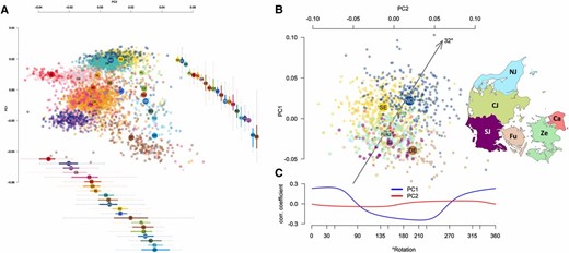
(A) PCA of 105,672 imputed SNPs after merging four data sets: Where Are You From?, POPRES, NCNG, and the Swedish Schizophrenia Study without outliers clustering with Finland (total N = 3858). Per-country box plots (median and interquartile range) of PC values were added to facilitate interpretation. Whiskers represent data within 1.5 times the interquartile range. IE: Ireland; ES: Spain; PT: Portugal; GB: Great Britain; FR: France; BE: Belgium; CH: Switzerland; NL: the Netherlands; DK: Denmark; DE: Germany; NO: Norway; SE: Sweden; AT: Austria; IT: Italy; PL: Poland; HU: Hungary; CZ: Czech Republic; HR: Croatia; RO: Romania; YU: Yugoslavia; GR: Greece. (B) PCA of 105,672 imputed SNPs from Denmark, Sweden, Norway and Germany with emphasis on the six geographic regions of Denmark (total N = 1168). No clear genetic–geographic relationship was observed. Ca: Capital; Ze: Zealand; Fu: Funen; SJ: South Jutland; CJ: Central Jutland; NJ: North Jutland. (C) Correlation of PC1 and PC2 with average grandparent place-of-birth latitude along a 360° Clockwise rotation. Maximum correlation was observed for PC1 at 32° (r ≈ 0.24; P < 10−5).
We then looked for fine-scale genetic structure within Denmark by focusing the analysis on 237 students who had at least three of their grandparents born in just one of the following six regions: Capital Region; Zealand; Funen; and South, Central, and North Jutland (Figure 2B). These six groups correspond to the five administrative regions of Denmark (we further split the administrative region of south Denmark into South Jutland and Funen). After rerunning PCA for Denmark, Sweden, Norway, and Germany alone (N = 1168), we observed no geographically meaningful clustering of the 237 Danish samples (Figure 2B). This lack of strong genetic structure was also supported by the low average FST value between the six regions (FST = 0.0002). To check whether structure was simply too weak to be visually detected, we calculated for each Danish sample the average geographic coordinates of their grandparents’ place of birth and regressed the resulting values on PC1 and PC2 eigenvectors. We repeated the procedure by gradually rotating the map clockwise and found a weak yet significant correlation between PC1 and latitude along a northwest–southeast axis at 32° (r ≈ 0.24; P < 10−5; Figure 2, B and C).
Chromosome painting, population clustering, and admixture
To further explore historical genetic interactions between Denmark and neighboring countries, we ran CHROMOPAINTER, fineSTRUCTURE, and GLOBETROTTER on a subset of the studied European populations. We used 2745 individuals from 13 European countries (Norway, Sweden, Finland, The Netherlands, Germany, Poland, Austria, Hungary, France, Belgium, Great Britain, Spain, and Portugal) and the 237 individuals from the six geographic regions in Denmark (Figure 1) to quantify and date European admixture in each of the six Danish groups. We used these six groups for our analysis because we were unable to observe an alternative clustering: fineSTRUCTURE clustered all Danish samples in a single large group (data not shown), reflecting again the weak genetic structure in the Danish population.
After running CHROMOPAINTER and fineSTRUCTURE on the European donor samples, these were organized in the eight major clusters seen in Figure 3A: Norwegian (NOR), Swedish (SWE), Finnish (FIN), British (BRI), French (FRA), German (GER), Polish (POL), and Iberian (IBE). There was always one predominant country in the makeup of each of those clusters, with the exception of IBE, in which Spain and Portugal were present at almost equal proportions, and GER, in which samples from Austria, Hungary, and The Netherlands were also present in large numbers. For convenience, we named the eight clusters after the predominant country/region in each of them. We treated these clusters as ancestry components (“surrogate populations” in GLOBETROTTER jargon) and used GLOBETROTTER to define their contribution to each of the six Danish regions and to date the corresponding admixture events.
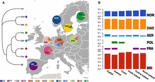
(A) fineSTRUCTURE grouping of the 2745 European donor samples into eight clusters roughly corresponding to well-defined geographic locations. The tree on the left illustrates cluster topology. Pie charts on the European map show the relative contribution from each country to each of the eight inferred clusters. FIN: Finnish; NOR: Norwegian; SWE: Swedish; POL: Polish; GER: German; BRI: British; FRA: French; IBE: Iberian. Color legend at the bottom of the map shows different donor countries. FI: Finland. (B) GLOBETROTTER admixture proportions of each of the eight European clusters in the six geographic regions of Denmark. Neither FIN nor IBE made substantial contributions (<2.5%) to the mixture profiles of Denmark.
Figure 3B and Table S2 show that the Swedish, Norwegian, and British clusters made the most substantial contribution to the ancestry profiles of all six Danish groups, jointly accounting for 82.05–97.12% of the total admixture. The Scandinavian component (Swedish and Norwegian clusters together) surprisingly accounted for less than half of the total admixture (range: 41.69–48.96%), on a par with the British component (40.37–48.16%), which peaked in South Jutland. Interestingly, the contribution of the Swedish cluster alone (27.45–30.20%) was almost twice as large as that of the Norwegian cluster (14.24–18.76%). This difference could be explained by the reduced landscape connectivity between Norway and Denmark, affecting gene flow patterns. It is also striking that the German cluster had little genetic influence on Denmark (3.04–6.78%), despite the proximity and historically fluid borders between the two countries. However, the latter observation could be due to the marginally higher genetic affinity of Denmark with Britain, which could result in prioritizing British over German samples in the initial chromosome-painting step of our analysis. Similarly, the French component was present at small yet considerable portions (4.16–5.42%) in all Danish regions except for Funen and South Jutland. Finally, it is worth noting that there was a small Polish contribution to Zealand (6.28%) and Funen (5.03%).
We further used GLOBETROTTER in a preliminary bootstrap resampling step within each of the six Danish regions to produce admixture dates. A proportion of nonsensical dates (i.e., ≤1 generation or ≥400 generations) above the empirical P-value threshold (0.05) suggests that GLOBETROTTER cannot date reliably the corresponding admixture event. Following this procedure, we found that we did not have enough power to date admixture in the Capital Region or in Funen (data not shown). For the remaining four regions, we used GLOBETROTTER’s pairwise coancestry curves (Figure S1, Figure S2, Figure S3, and Figure S4) to define in more detail the type (i.e., one date vs. one date multiway vs. two dates) and actual date of admixture, as well as a tentative composition of the admixing source populations. In all regions, GLOBETROTTER’s best fitting admixture model (R2 = 0.136–0.354) involved one admixture event with more than two sources admixing simultaneously (Table 1). Assuming 30 years per generation, the date of admixture ranged from ∼434 to ∼943 years before present. Notably, the algorithm identified two clusters as the most recurring admixing sources: one showing highest affinity with GER and one with POL.
Summary of GLOBETROTTER’s inference of the date of admixture and composition of admixing sources for each of four geographic regions of Denmark
| Admixture event 1 | Admixture event 2 | |||||||||
|---|---|---|---|---|---|---|---|---|---|---|
| Region | Best fitting type of admixture | Goodness of fit (R2) | Years before present (95% CI) | Year | Minor component | Major component | Ratio | Minor component | Major component | Ratio |
| Zealand (N = 36) | 1 date multiway | 0.208 | 943 (579, 1488) | 1052 | BRI | SWE | 0.47:0.53 | GER | POL | 0.47:0.53 |
| S. Jutland (N = 37) | 1 date multiway | 0.136 | 756 (232, 1548) | 1239 | FRA | POL | 0.21:0.79 | GER | POL | 0.43:0.57 |
| C. Jutland (N = 89) | 1 date multiway | 0.354 | 611 (418, 823) | 1384 | BRI | POL | 0.31:0.69 | POL | GER | 0.45:0.55 |
| N. Jutland (N = 48) | 1 date multiway | 0.239 | 434 (118, 741) | 1561 | BRI | POL | 0.33:0.67 | GER | POL | 0.42:0.58 |
Type of admixture was chosen among three alternatives: (i) one date, (ii) one date multiway, and (ii) two or more dates. Multiway admixture involves two admixture events. If a source population appears in both admixture events 1 and 2, then the interpretation is “three-way admixture” (for more details see Busby et al. 2015). R2: goodness of fit for a single date of admixture, taking the maximum value across all inferred coancestry curves (R2 ≥ 0.2 corresponds to good fit). GLOBETROTTER returns date estimates in generations. We multiplied these estimates by 30 years/generation. We retrieved historical dates by subtracting year estimates from 1995 (the median year of birth for our high school students). CI: confidence interval.
| Admixture event 1 | Admixture event 2 | |||||||||
|---|---|---|---|---|---|---|---|---|---|---|
| Region | Best fitting type of admixture | Goodness of fit (R2) | Years before present (95% CI) | Year | Minor component | Major component | Ratio | Minor component | Major component | Ratio |
| Zealand (N = 36) | 1 date multiway | 0.208 | 943 (579, 1488) | 1052 | BRI | SWE | 0.47:0.53 | GER | POL | 0.47:0.53 |
| S. Jutland (N = 37) | 1 date multiway | 0.136 | 756 (232, 1548) | 1239 | FRA | POL | 0.21:0.79 | GER | POL | 0.43:0.57 |
| C. Jutland (N = 89) | 1 date multiway | 0.354 | 611 (418, 823) | 1384 | BRI | POL | 0.31:0.69 | POL | GER | 0.45:0.55 |
| N. Jutland (N = 48) | 1 date multiway | 0.239 | 434 (118, 741) | 1561 | BRI | POL | 0.33:0.67 | GER | POL | 0.42:0.58 |
Type of admixture was chosen among three alternatives: (i) one date, (ii) one date multiway, and (ii) two or more dates. Multiway admixture involves two admixture events. If a source population appears in both admixture events 1 and 2, then the interpretation is “three-way admixture” (for more details see Busby et al. 2015). R2: goodness of fit for a single date of admixture, taking the maximum value across all inferred coancestry curves (R2 ≥ 0.2 corresponds to good fit). GLOBETROTTER returns date estimates in generations. We multiplied these estimates by 30 years/generation. We retrieved historical dates by subtracting year estimates from 1995 (the median year of birth for our high school students). CI: confidence interval.
Ancestry component analysis
We also used Ohana to provide an independent estimate of individual admixture proportions in the same set of 12 European countries (without Finland) and six Danish regions. For this purpose, we assumed that each of the European samples was the result of admixture between K ancestral populations (i.e., ancestry components). Even though we ran the analysis for K = {2, …, 9} (Figure S5), we report the results for K = 4, because this value corresponds to four distinct geographic origins of our samples: the Iberian Peninsula and Eastern, Central, and Nordic Europe. The analysis returned an admixture pattern that was consistent with geography (i.e., north–south and east–west clines; Table 2 and Figure 4). In particular, we observed (i) a Southern European component (blue), which was predominant in the Iberian Peninsula but was also found at large proportions in France; (ii) an Eastern European component (yellow), which was predominant in Poland but was also found at large proportions in neighboring countries (and notably in south and east Denmark, Sweden, Norway, and Great Britain); (iii) a nordic component (green), which was predominant in Scandinavia and to a lesser extent in Germany; and (iv) a Central European component (red), at higher proportions in Scandinavia and The Netherlands but also present in most European countries (except for Iberia). Within Denmark, we observed that Zealand and south Denmark had larger membership to the Eastern European component (18.90–20.36%) compared to Central and North Jutland (∼13%), resembling GLOBETROTTER’s signal of Polish admixture observed in Zealand and Funen (Figure 3B and Table S2). The Southern and Eastern European components were robust to different choices of K, whereas the Central and Nordic European components were gradually divided into smaller fractions as K went up, showing no clear geographic patterns (Figure S5).
Percentage of membership of 13 European countries (including six well-defined geographic regions in Denmark shown in the inset) to each of K = 4 ancestral populations
| Ancestral component | ||||
|---|---|---|---|---|
| Country/region | % Southern (blue) | % Eastern (yellow) | % Central (red) | % Nordic (green) |
| PT | 72.43 | 8.59 | 12.15 | 6.83 |
| ES | 78.32 | 3.57 | 9.25 | 8.86 |
| FR | 45.70 | 15.19 | 19.23 | 19.88 |
| BE | 35.64 | 14.06 | 20.84 | 29.46 |
| GB | 30.08 | 32.28 | 15.20 | 22.45 |
| NL | 24.88 | 20.06 | 23.62 | 31.44 |
| DE | 23.10 | 17.22 | 22.40 | 37.28 |
| AT | 20.28 | 17.44 | 19.88 | 42.39 |
| HU | 29.41 | 49.76 | 11.83 | 9.00 |
| PL | 3.59 | 76.19 | 9.83 | 10.38 |
| Ca | 5.39 | 21.27 | 24.94 | 48.40 |
| Ze | 7.73 | 18.90 | 25.67 | 47.71 |
| Fu | 6.51 | 20.36 | 28.28 | 44.85 |
| SJ | 5.94 | 19.49 | 28.94 | 45.64 |
| CJ | 7.34 | 13.35 | 30.30 | 49.01 |
| NJ | 5.82 | 13.23 | 32.35 | 48.60 |
| NO | 8.56 | 13.24 | 30.91 | 47.29 |
| SE | 4.98 | 17.39 | 27.27 | 50.35 |
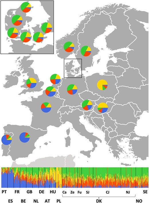
Ancestral component analysis of 13 European countries (including six well-defined geographic regions in Denmark shown in the inset) assuming K = 4 ancestral populations. Bar plot at the bottom shows per-individual membership to each of the four ancestral components, whereas pie charts on the map resume per-country (or per-region for Denmark) admixture proportions. Based on their preponderance in different parts of Europe, we interpret the four components as (i) Southern European (blue); (ii) Eastern European (yellow); (iii) Nordic (green); and (iv) Central European (red). Regions from south and east Denmark show higher proportion of Eastern European ancestry in accord with Figure 3B and Table S2.
Relatedness and IBD
We followed up the evidence for weak genetic structure in Denmark by exploring the degree and geographic distribution of relatedness among our Danish samples. Using KING, we found that the vast majority of the Danish students were distantly related (fourth degree or more distant), with only four pairs of individuals showing second or third degree relationships (apart from the twins and siblings initially removed; Figure S6). Because of the inherent uncertainty in distinguishing between different degrees of distantly related individuals, we did not attempt to further stratify the samples by kinship coefficient.
After establishing that most participants in our sample were either unrelated or distantly related (Figure S6), we examined DNA segments that were IBD between pairs of individuals with BEAGLE Refined IBD. Using total genomic length of IBD tracts as a proxy for relatedness, we traced each individual’s closest “genomic relative” within Denmark without explicitly quantifying the degree of relationship. Figure 5A shows the distribution of the geographic distance of each of 399 individuals from their closest genomic relative (pink) and from a randomly chosen sample (green). The distribution of the distance from the closest relative (pink) showed an enrichment for very short distances, i.e., less than ∼50 km, as well as a median value of 99.3 km—significantly closer than expected by chance at 131.4 km (Mann–Whitney U = 60,997; P < 10−8). This points at a weak yet significant tendency of participants to live close to genetically similar individuals.
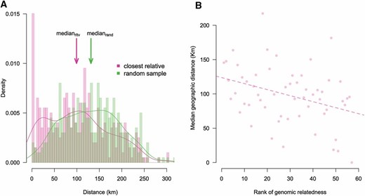
(A) Distribution of geographic distance of each participant’s place of birth (N = 399) to that of their closest “genomic relative” (pink) and to that of a randomly chosen sample (green). Genomic relatedness was defined on the grounds of total genomic IBD. Arrows point at median values of the two distributions (medianrltv = 99.3 km; medianrand = 131.4 km). Seven individuals with unknown geographic coordinates were excluded from this analysis. (B) Plot of rank of genomic relatedness vs. median geographic distance of each participant to their closest genomic relative. We created 57 equally sized bins of individuals increasingly related to their closest genomic relative (seven individuals per bin). Alternative bin sizes also produced significantly negative correlations (data not shown).
To gain more insight into the latter observation, we grouped our Danish samples into ranked bins by the amount of total genomic IBD shared with their closest genomic relative (the higher the rank, the closer the relationship). We then calculated the median geographic distance of each participant to their closest relative within each bin and regressed this value against bin rank (Figure 5B) to observe a weak yet significant negative correlation (r ≈ −0.35; P < 0.01). This observation points out that geographic distance tends to be significantly shorter between Danes who share more genomic IBD. Interestingly, this signal was not picked up by kinship coefficient (data not shown).
Historical effective population size
Historical Ne showed notable disparity between the three Scandinavian countries (Figure 6). In particular, point estimates of Ne in Denmark, Norway, and Sweden showed a dramatic ∼273-fold, ∼262-fold, and ∼995-fold increase over the past 150 generations (∼4500 ± 300 years), following the general upward European trend (Browning and Browning 2015). What is more, Sweden’s and Denmark’s Ne estimates were significantly different from each other (no overlap between the corresponding 95% confidence intervals). During the High and Late Middle Ages, Ne in Denmark remained stable, suffering an almost imperceptible decline as a consequence of the otherwise devastating Black Death and similar patterns were observed for Norway and Sweden. From the 15th century on, Ne in Denmark started to rise again at a moderate rate, whereas Ne in Norway and Sweden rose at an even higher rate, resulting in Norway’s Ne eventually surpassing that of Denmark. Interestingly, even though Denmark and Norway currently have very similar census population sizes (5.614 and 5.084 million, respectively), Norway’s current Ne is 1.76 times larger than Denmark’s (even though not significantly different). Finally, the upward trend of Denmark’s Ne did not seem to be withheld by other important epidemics in the history of the country, such as cholera, the Spanish flu, or, more recently, polio (Figure 6).
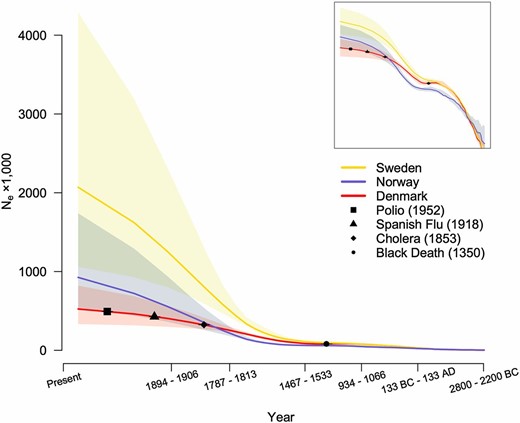
Change in effective population size (Ne) of the Danish, Swedish, and Norwegian populations over the past 150 generations (log scale). Shaded areas represent the upper and lower bounds of the 95% confidence intervals after bootstrapping. Uncertainty in generation length is represented by year intervals on the x-axis, assuming that each generation lasts 30 ± 2 years. Black segments represent major epidemics from the recent history of the Danish population and are plotted taking into account generation length uncertainty. For more clarity, the inset shows the same graph with both axes in log scale.
Polygenic prediction of height and BMI
Polygenic risk prediction in our Danish sample was overall far more accurate for height than for BMI (Figure S7). In the case of height, we observed maximum accuracy when assuming infinitesimal genetic architecture and adjusting for age, sex, and 10 ancestry PCs—R2 = 0.251 ± 0.031 (Figure S7A) vs. ∼0.17 elsewhere (Wood et al. 2014). When age, sex, and the 10 PCs were also included in the model, the prediction rose substantially to 0.639 ± 0.015 (P = 6.57 × 10−71), a fact reflected in the strong and significant correlation between real and predicted height (Figure S7C). In contrast, although the maximum accuracy of BMI prediction was also observed when we adjusted for age, sex, and 10 PCs, this was overall much poorer than for height—R2 = 0.106 ± 0.037 (Figure S7B) vs. ∼0.065 elsewhere (Locke et al. 2015). In this case, when age, sex, and 10 PCs were included in the model, the improvement of accuracy was not as notable as for height (R2 = 0.195 ± 0.034, P = 5.49 × 10⁻¹⁸), implying that BMI is only marginally affected by age and sex (Figure S7D).
Discussion
The most notable observation of our study is the high genetic homogeneity of the Danish population, possibly reflecting geographically uninterrupted gene flow, further facilitated by the extended network of sea-based commerce and traveling (Derry 2000). This observation should be appreciated in a historical context, as our analysis did not account for genetic contributions from recent immigration. Indeed, modern Danish society accommodates different ethnic and cultural groups (Jensen and Pedersen 2007), and this was also reflected in our sample, where ∼4% of the participants were born in Afghanistan, China, Ethiopia, Finland, Germany, Greenland, Iraq, Jordan, Korea, Kosovo, The Netherlands, or Zambia. This number went up when we looked at grandparental origin, where 14.6% of the participants had at least one grandparent born outside Denmark.
The historical homogeneity of the Danish population is reflected in the lack of PCA clustering (Figure 2B), as well as in the notably low average FST between the six geographic regions. To put this observation in context, a previous study was able to detect subtle population structure along a north–south axis in The Netherlands (Genome of the Netherlands Consortium 2014), a country of almost identical area to Denmark’s. Even though we were able to detect significant correlation between PC1 and latitude (Figure 2C), the signal was less compelling than that from the Dutch study. Similarly, a recent study of population structure in Great Britain (Leslie et al. 2015) found that the average pairwise FST estimates between 30 geographic regions was 0.0007—3.5 times higher than the value we report here (0.0002).
To better understand how our FST estimates compare to those from Great Britain, we calculated average FST values in two British population sets using FST values reported elsewhere (Leslie et al. 2015). The two British sets included regions with geographic distances comparable to those in Denmark. The first subset composed of 13 populations from central/southern England with a resulting average FST < 0.0002. The second subset composed of nine populations from northern England with a resulting average pairwise FST = 0.0003.
In general, the study of admixture within the European continent is confounded by a well-grounded isolation-by-distance mechanism (Lao et al. 2008; Novembre et al. 2008), as well as an increased historical complexity that renders most admixture models unrealistically simple (Busby et al. 2015). Denmark is no exception to these caveats. Even though it is tempting to explain the admixture proportions in Figure 3 and Figure 4 as the result of historical admixing events, an alternative approach is to interpret such proportions as “mixture profiles.” Bearing this in mind, we see that the mixture profiles of all six Danish groups comprise two major ancestry components, one predominant in Scandinavia and the other predominant in Central Europe (Figure 4). In the GLOBETROTTER analysis, these two components were identified as admixture contributions from the Swedish/Norwegian and the British clusters (Figure 3B and Table S2). In regard to the British contribution, however, this is actually more likely to reflect admixture in the opposite direction, i.e., from Denmark to Britain (Leslie et al. 2015).
Even though the mixture profiles of the six regions in Denmark were overall quite similar, they differed in their membership to the Eastern European cluster. This particular cluster was more prevalent in south and east Denmark (Figure 4) and was independently observed in the GLOBETROTTER analysis as a small Polish contribution to Zealand and Funen (Figure 3B and Table S2). This signal could be due to historical Wend settlements in the broader area around Lolland in the southernmost part of Denmark (Derry 2000), an observation that is also supported by our admixture date estimates (Table 1). However, because similar mixture profiles were also observed in Sweden and Norway (Figure 4), it is difficult to choose between isolation by distance and actual admixture.
Given the high variance in the estimated admixture dates, the recurrence of the same combinations of admixing sources, and the largely unstructured nature of our Danish sample, we could interpret several of the admixture patterns in Table 1 as different instances of the same event. For instance, focusing on the two surrogates that GLOBETROTTER found best tagged by POL and GER, we see that the admixture between them first occurred in Zealand in the 11th century, spreading to the rest of peninsular Denmark afterward. This observation fits historical knowledge about the march of the Wends toward Denmark, as mentioned above.
A weak signal of population structure was also observed when we studied the geographic distribution of IBD-based relatedness. The median distance to the closest genomic relative was significantly smaller than to a randomly chosen sample, but it represents a minor effect (median difference ≈ 30 km; Figure 5A). In our regression analysis, we observed that this distance tended to be significantly smaller for pairs of individuals that were more identical, yet the correlation was overall modest (r ≈ −0.35; Figure 5B). These observations point out that genetic structure indeed exists in Denmark, even though it is very weak.
It is striking that Denmark, Sweden, and Norway—three closely related Scandinavian countries—seem to differ considerably in their demographic history, as reflected in their historical Ne trajectories (Figure 6). Indeed, current Sweden-to-Norway census population size ratio is 1.89—considerably close to their current Ne ratio (2.24)—implying that the two populations have had similar reproductive variance and/or population structure. On the contrary, Denmark’s Ne seems to have increased at a consistently lower rate after the Middle Ages. This could be reflecting weaker reproductive dynamics in the Danish population or weaker population structure compared to Sweden and Norway. Larger sample sizes are warranted to shed more light on the historical Ne trajectories in Scandinavian populations.
Finally, we found that self-reported adolescent height could be predicted with remarkable accuracy using essentially nothing but information derived directly (genotypes) or indirectly (sex and ancestry) from DNA available at birth. When we combined SNP data with age, sex, and PCA information, our predictor could explain more than half of the total phenotypic variance (63.9%). The remaining unexplained variance corresponded to a standard deviation of 5.43 cm. This means that, with 95% confidence, we are at most ∼10.65 cm off in our prediction of adolescent height (Figure S7C). It is worth noting that adding age to the model did not yield significant improvements to the prediction accuracy of height (data not shown), implying that adolescent height is a reliable measurement for the validation of the prediction. In addition, even though height was a self-reported measurement, its strong correlation with predicted adult height suggests that the students provided reliable personal information (Figure S7C). As for the poorer prediction of BMI, it is important to remember that data training was carried out in adults, whereas prediction was validated in adolescents. Therefore, further improvement of the BMI prediction as subjects advance in age is a possibility.
In conclusion, our analysis showed that, by applying the simple criterion of participants having all four of their grandparents born in Denmark, we obtained a largely unstructured sample with very low FST values among different geographic regions. This high homogeneity has the potential of rendering population structure in large-scale Danish gene-mapping studies such as iPSYCH (http://ipsych.au.dk/) a lesser concern, regardless of adjustments such as genomic control (Devlin and Roeder 1999), PCA (Price et al. 2006), or mixed models (Yu et al. 2006). We also observed a notably disparate demographic history in Demark compared to other Scandinavian countries—a fact that can also be ascribed to the high homogeneity of the Danish population—and that height in adolescents could be predicted with considerable accuracy. Lastly but not least importantly, this study stands as an example of how large-scale public engagement projects can provide mutual benefits for both the general public and the scientific community through the promotion of scientific knowledge.
Acknowledgments
The authors thank the high school students and their teachers for participating in the Where Are You From? project, as well as Dagmar Hedvig Fog Bjerre and Pia Johansson Nielsen for logistic support with organizing and shipping the DNA kits to the participating schools. Special thanks to Jes Fabricius Møller for helping us gain useful insights into the history and demography of the Danish population. G.A. thanks Garrett Hellenthal, Francesco Montinaro, George Busby, Sharon Browning, and Christopher Gignoux for their help and useful discussions. This project and related research were supported by the National Lottery Funds (Danske Spil), the Danish Ministry of Education, and the Centre for Biocultural History, Aarhus University. B.J.V. was supported by a grant from the Danish Council for Independent Research (DFF-1325-0014). C.M.H. was supported by grants from the Swedish Research Council (K2014-62X-21445-05-3 and K2012-63X-21445-03-2).
Footnotes
Communicating editor: R. Nielsen
Supplemental material is available online at www.genetics.org/lookup/suppl/doi:10.1534/genetics.116.189241/-/DC1.
Literature Cited
Derry, T. K., 2000 History of Scandinavia: Norway, Sweden, Denmark, Finland, and Iceland. University of Minnesota Press, Minneapolis.
Author notes
Present address: Natural History Museum of Denmark, University of Copenhagen, Copenhagen, 1471, Denmark.
