


ABSTRACT
We have constructed a series of nonrotating quasi-hydrostatic evolutionary models for the M2 Iab supergiant Betelgeuse (α Orionis). Our models are constrained by multiple observed values for the temperature, luminosity, surface composition, and mass loss for this star, along with the parallax distance and high-resolution imagery that determines its radius. We have then applied our best-fit models to analyze the observed variations in surface luminosity and the size of detected surface bright spots as the result of up-flowing convective material from regions of high temperature in the surface convective zone. We also attempt to explain the intermittently observed periodic variability in a simple radial linear adiabatic pulsation model. Based on the best fit to all observed data, we suggest a best progenitor mass estimate of  and a current age from the start of the zero-age main sequence of 8.0–8.5 Myr based on the observed ejected mass while on the giant branch.
Export citation and abstract BibTeX RIS
1. INTRODUCTION
The M2 Iab supergiant Betelgeuse (α Orionis) is an ideal laboratory to study advanced stages of stellar evolution. It has the largest angular diameter of any star apart from the Sun and is one of the brightest M giants. As such, it has been well studied. Direct Hubble Space Telescope imagery exists for this star (Gilliland & Dupree 1996; Lobel & Dupree 2001; Dupree & Stefanik 2013), as well as other high-resolution indirect imagery (Balega et al. 1982; Buscher et al. 1990; Marshall et al. 1992; Wilson et al. 1992, 1997; Burns et al. 1997; Haubois et al. 2009; Ohnaka et al. 2009; Townes et al. 2009; Ohnaka 2013, 2014). Both the light curve and the imagery indicate the appearance of intermittent bright spots associated with irregular variability in the star's luminosity and temperature. The chromosphere has exhibited (Dupree et al. 1987; Dempsey 2015) a periodic (∼420 day) modulation in the optical and UV flux most likely associated with photospheric pulsations that later became substantially weaker and disappeared (Dupree & Stefanik 2013). The star is classified (Samus et al. 2011) as a semiregular variable with an SRC subclassification with a period of 2335 days (6.39 yr).
A shell of circumstellar material has also been detected around this star (Noriega-Crespo et al. 1997; Lobel & Dupree 2001; Lobel 2003a, 2003b), and it appears to be losing mass at a rate of ∼(1–3) × 10−6 M⊙ yr−1 (Knapp & Morris 1985; Glassgold & Huggins 1986; Bowers & Knapp 1987; Skinner & Whitmore 1987; Mauron 1990; Marshall et al. 1992; Young et al. 1993; Huggins et al. 1994; Mauron & Guilain 1995; Guilain & Mauron 1996; Harper et al. 2001, 2008; Plez & Lambert 2002; Ryde et al. 2006; Le Bertre et al. 2012; O'Gorman et al. 2015; Kervella et al. 2016).
Isotopic CNO abundance data that suggest evidence of deep interior mixing are also available (Gautier et al. 1976; Harris & Lambert 1984; Lambert et al. 1984). On the other hand, this star exhibits a slow rotation velocity of  km s−1 and an inclination of
  (Gilliland & Dupree 1996; Kervella et al. 2009), implying a rotation period of 8.4 yr. Hence, rotation may not significantly affect the interior structure at the present time, although it is likely to have affected the main-sequence evolution (Meynet et al. 2013).
These measurements have been complemented by the availability of high-precision parallax measurements from the Hipparcos satellite (ESA 1997; Perryman et al. 1997; van Leeuwen 1997; Kovalevsky 1998), which have been revised (Harper et al. 2008). The absolute luminosities and photospheric radii are now sufficiently well determined to warrant a new investigation of the constraints on models for this star.
In spite of this accumulated wealth of information, there have been only a few attempts (e.g., Meynet et al. 2013) to apply a stellar evolution calculation in sufficient detail to explore the implications of these observed properties on models for the advanced evolution of this massive star. Here we complement other such studies with an independent application of two quasi-static stellar evolution codes from the pre-main sequence through the star's lifetime. We have made a search to find the combinations of mass, mixing length, mass-loss history, and age that best reproduce the observed radius, temperature, luminosity, current mass-loss rate, and observed ejected mass for this star. We then study the observed brightness variations, surface abundances, surface turbulent velocities, and periodicity in the context of this model. We find that both the observed intermittent periodicity and the hot-spot variability are plausible outcomes of the surface convective properties of the model.
2. DATA
Over the years a great deal of data have accumulated for α Orionis (see Kervella et al. 2013a, and references therein). Tables 1–5 summarize some of the observations and our adopted constraints as discussed below.
Table 1. Summary of Astronometric and Distance Data for Betelgeuse
| Ref. | p (mas) | Distance (pc) | vrad (km s−1) |  |
μδ |
|---|---|---|---|---|---|
| Stanford (1933) | ⋯ | ⋯ | 20.7 ± 0.4 | ⋯ | ⋯ |
| Lambert et al. (1984) | ⋯ | 155 | ⋯ | ⋯ | ⋯ |
| Hipparcos ESA (1997) | 7.63 ± 1.64 |  |
⋯ | 27.33 ± 2.30 | 10.86 ± 1.46 |
| Tycho ESA (1997) | 18.6 ± 3.6 |  |
⋯ | ⋯ | ⋯ |
| Famaey et al. (2005) | ⋯ | ⋯ | 21.91 ± 0.51 | ⋯ | ⋯ |
| Harper et al. (2008) | 5.07 ± 1.10 | 197 ± 45 | ⋯ | 24.95 ± 0.08 | 9.56 ± 0.15 |
| Adopted | 5.07 ± 1.10 | 197 ± 45 | 21.91 ± 0.51 | 24.95 ± 0.08 | 9.56 ± 0.15 |
Download table as: ASCIITypeset image
2.1. Distance
In spite of its brightness, confusion in the proper motion, variability, asymmetry, and large angular diameter have together made the determination of the distance to this star difficult. A summary of the astrometric data is presented in Table 1. The first parallax distance measurements reported by Hipparcos (∼131 pc) and Tycho (∼54 pc) disagreed by more than a factor of two (ESA 1997). This was well outside the range of quoted errors. However, the more recent VLA-Hipparcos distance to Betelgeuse of ∼197 ± 45 pc (Harper et al. 2008) has been derived from multiwavelength observations. This is the value adopted here as having the greatest accuracy and least distortion from the variability.
2.2. Luminosity and Temperature
Because of the variability of the star during observations, it is difficult to ascribe a mean value and uncertainty to the visual magnitude, luminosity, and temperature. The error bars associated with the quoted apparent visual magnitudes and temperatures in Table 2 are largely a measure of the intrinsic variability of the star. They are therefore not a true measurement error. Hence, to assign an uncertainty to the adopted mean visual magnitudes and temperatures, we simply take the unweighted standard deviation of the various determinations of the mean value. Since the luminosity depends on distance, we simply adopt the luminosity of Harper et al. (2008) based on the revised Hipparcos distance in that paper.
Table 2. Summary of Luminosity Temperature Data for Betelgeuse
| Reference | V |  |
Teff (K) |
|---|---|---|---|
| Lee (1970) | 0.4 | ⋯ | ⋯ |
| Wilson (1976) | 0.7 | ⋯ | ⋯ |
| Sinnott (1983) | 0.5 ± 0.6 |  |
⋯ |
| Lambert et al. (1984) | ⋯ | ⋯ | 3800 ± 100 |
| Cheng et al. (1986) | 0.42 | ⋯ | ⋯ |
| Gaustad (1986) | ⋯ | ⋯ |  |
| Mozurkewich et al. (1991) | 0.5 | ⋯ | ⋯ |
| Dyck et al. (1992) | 0.32 ± 0.24 |  |
3520 ± 85 |
| Krisciunas (1992) | 0.43 ± 0.14 |  |
⋯ |
| Di Benedetto (1993) | ⋯ | ⋯ | 3620 ± 90 |
| Bester et al. (1996) | ⋯ | ⋯ | 3075 ± 125 |
| Krisciunas & Luedeke (1996) | 0.59 ± 0.24 |  |
⋯ |
| Dyck et al. (1996, 1998) | ⋯ | ⋯ | 3605 ± 43 |
| Wilson et al. (1997) | 0.64 ± 0.20 |  |
⋯ |
| Perrin et al. (2004) | ⋯ | 4.80 ± 0.19 | 3641 ± 53 |
| Ryde et al. (2006) | ⋯ | ⋯ | 3250 ± 200 |
| Harper et al. (2008) | ⋯ | 5.10 ± 0.22 | ⋯ |
| Ohnaka et al. (2011) | ⋯ | ⋯ | 3690 ± 54 |
| Adopted |  |
5.10 ± 0.22 | 3500 ± 200 |
Download table as: ASCIITypeset image
2.3. Angular Diameter
Determinations of the angular diameter Θdisk and associated radius of this star from the observations are summarized in Table 3. This is also complicated by various factors. Red supergiants (RSGs) like α Orionis are extended in radius. As such, their surface gravity is smaller than a main-sequence star like the Sun. This results in extended atmospheres and large convective motion that produces asymmetry along with variability in the surface temperature and luminosity. In addition to the random variability in surface luminosity and temperature and intermittent periodic variability, the diameter of this star seems to change with time (Townes et al. 2009).
Table 3. Summary of Angular Diameter/Radius Data for Betelgeuse
| Ref. | Year Obs. | λ (μm) |  |
 |
R/R⊙ |
|---|---|---|---|---|---|
| Michelson & Pease (1921) | 1920 | 0.575 | 47.0 ± 4.7 | 55 ± 7 | ⋯ |
| Balega et al. (1982) | 1978 | 0.405–0.715 | 56 ± 11 | 57 ± 7 |  |
| 1979 | 0.575–0.773 | 56 ± 6 | 57 ± 7 |  |
|
| Cheng et al. (1986) | ⋯ | ⋯ | 42.1 ± 1.1 | ⋯ |  |
| Buscher et al. (1990) | 1989 | 0.633–0.710 | 57 ± 2 | ⋯ |  |
| Mozurkewich et al. (1991) | ⋯ | ⋯ | ⋯ | 49.4 ± 0.2 |  |
| Dyck et al. (1992) | ⋯ | ⋯ | ⋯ | 46.1 ± 0.2 |  |
| Wilson et al. (1992) | 1991 | ⋯ | ⋯ | 54 ± 2 |  |
| Bester et al. (1996) | ⋯ | ⋯ | ⋯ |  |
⋯ |
| Dyck et al. (1996, 1998) | ⋯ | ⋯ | ⋯ | 44.2 ± 0.2 | ⋯ |
| Burns et al. (1997) | ⋯ | ⋯ | ⋯ | 51.1 ± 1.5 | ⋯ |
| Tuthill et al. (1997) | ⋯ | ⋯ | ⋯ | 57 ± 8 |  |
| Wilson et al. (1997) | ⋯ | ⋯ | ⋯ | 58 ± 2 |  |
| Weiner et al. (2000) | 1999 | 11.150 | 54.7 ± 0.3 | 55.2 ± 0.5 | ⋯ |
| Perrin et al. (2004) | 1997 | 2.200 | 43.33 ± 0.04 | 43.76 ± 0.12 | 620 ± 124 |
| Perrin et al. (2004) | ⋯ | 11.15 | 55.78 ± 0.04 | 42.00 ± 0.06 | 620 ± 124 |
| Haubois et al. (2009) | 2005 | 1.650 | 44.3 ± 0.1 | 45.01 ± 0.12 | ⋯ |
| Neilson et al. (2012) | 2005 | 1.650 | ⋯ | 44.93 ± 0.15 | 955 ± 217 |
| Hernandez-Utrera & Chelli (2009) | 2006 | 2.009–2.198 | 42.57 ± 0.02 | ⋯ | ⋯ |
| Tatebe et al. (2007) | ⋯ | ⋯ | 48.4 ± 1.4 | ⋯ | ⋯ |
| Ohnaka et al. (2009) | 2008 | 2.28–2.31 | 43.19 ± 0.03 | ⋯ | ⋯ |
| Townes et al. (2009) | 1993.83 | 11.150 | 56.0 ± 1.0 | ⋯ | ⋯ |
| 1994.60 | 11.150 | 56.0 ± 1.0 | ⋯ | ⋯ | |
| 1999.875 | 11.150 | 54.9 ± 0.3 | ⋯ | ⋯ | |
| 2000.847 | 11.150 | 53.4 ± 0.6 | ⋯ | ⋯ | |
| 2000.917 | 11.150 | 55.8 ± 0.9 | ⋯ | ⋯ | |
| 2000.973 | 11.150 | 54.8 ± 1.0 | ⋯ | ⋯ | |
| 2001.64 | 11.150 | 53.4 ± 0.6 | ⋯ | ⋯ | |
| 2001.83 | 11.150 | 52.9 ± 0.4 | ⋯ | ⋯ | |
| 2001.97 | 11.150 | 52.7 ± 0.7 | ⋯ | ⋯ | |
| 2006.91 | 11.150 | 48.4 ± 1.4 | ⋯ | ⋯ | |
| 2007.96 | 11.150 | 50.0 ± 1.0 | ⋯ | ⋯ | |
| 2008.09 | 11.150 | 49.0 ± 1.5 | ⋯ | ⋯ | |
| 2008.83 | 11.150 | 47.0 ± 2.0 | ⋯ | ⋯ | |
| 2008.93 | 11.150 | 47.0 ± 1.0 | ⋯ | ⋯ | |
| 2009.05 | 11.150 | 48.0 ± 1.0 | ⋯ | ⋯ | |
| 2009.09 | 11.150 | 48.0 ± 2.0 | ⋯ | ⋯ | |
| Ohnaka et al. (2011) | 2009 | 2.28–2.31 | 42.05 ± 0.05 | 42.09 ± 0.06 | ⋯ |
| Adopted | ⋯ | ⋯ | 55.64 ± 0.04 | 41.9 ± 0.06 | 887 ± 203 |
Download table as: ASCIITypeset image
Interferometric measurements can be used to determine an effective uniform disk diameter. However, measurements made at one wavelength must be corrected for the variation in the optical depth with wavelength to yield an effective Rosseland mean radius to compare with the Rosseland radius computed in stellar models.
One must also correct the inferred disk for effects of limb darkening, which tend to diminish the observed radius relative to the Rosseland mean radius. This correction can be of order 10% in visible wavelengths or only as little as ∼1% in the near-infrared (Weiner et al. 2002). The presence of hot spots also tends to diminish the apparent radius (Weiner et al. 2003) by as much as 15%. Moreover, the surrounding circumstellar envelope and dust also complicate the identification of the edge of the star. Furthermore, measurements at different wavelengths lead to different results. Infrared measurements over the past 15 yr even seemed to indicate (Townes et al. 2009) that the radius of this star has been recently systematically decreasing (see, however, Ohnaka 2013).
As a result of all of these complications, one must exercise caution when using measurements of the angular diameter. In Table 3 we quote (when available) the uniform disk Rossland mean radius corrected for limb darkening. Quoted values in the literature are distributed into two distinct groups roughly depending on wavelength. One group λ ∼ 1 μm) is centered around 44 mas (Cheng et al. 1986; Mozurkewich et al. 1991; Dyck et al. 1992; Perrin et al. 2004; Haubois et al. 2006, 2009), while the other ( ) is centered around 57 mas (Balega et al. 1982; Buscher et al. 1990; Wilson et al. 1992, 1997; Bester et al. 1996; Burns et al. 1997; Tuthill et al. 1997; Weiner et al. 2000).
Photospheric radii must be corrected for limb darkening and wavelength. These corrections are the smallest for the 11 μm measurements (Weiner et al. 2000). Hence, we adopt a weighted average of the 11.15 μm measurements to obtain 55.6 ± 0.04 mas, which would lead to a photospheric Rosseland mean radius of 56.2 ± 0.04 mas.
However, it is argued quite persuasively in Perrin et al. (2004) that the discrepancy between the lower and higher radii could be accounted for in a unified model that includes the possibility of a warm molecular layer around the star, consistent with that also observed in Mira variables. Applying this correction to the 11.15 μm data leads to a 75% correction (Perrin et al. 2004). This reduces the corrected angular diameter to 41.9 ± 0.04 mas. We adopt this as the best means to deduce a radius to compare with stellar models. This adopted angular diameter, combined with the VLA-Hipparcos distance and uncertainty of 197 ± 45 pc, yields a radius of 887 ± 203 R⊙. These parameters, along with the observed CNO abundances, lack of s-process abundances (Lundqvist & Wahlgren 2005), and the ejected mass, allow for constraints on stellar models as described below.
2.4. Surface Composition
The surface elemental and isotopic abundances adopted in this study are summarized in Table 4. Surface elemental C, N, and O abundances for Betelgeuse abundances have been measured by Lambert et al. (1984), while 12C/13C, 16O/17O, and 16O/18C isotopic ratios have been reported in Harris & Lambert (1984). As noted in those papers and in the calculations reported here, relative to the Sun, Betelgeuse has an enhanced nitrogen abundance, low carbon abundance, and low 12C/13C ratio. This is consistent with material that has been mixed to the surface as a result of the first dredge-up phase. As we shall see, this places a constraint on the location of this star on its evolutionary track, i.e., that it must have passed the base of the red giant branch (RGB) and is ascending the RSG phase.
Table 4. Composition Data for Betelgeuse
| Quantity | Ref. | ||
|---|---|---|---|
| [Fe/H] = +0.1 | Lambert et al. (1984) | ||
| X⊙ | Y⊙ | Z⊙ | |
| 0.71 | 0.27 | 0.020 | Anders & Grevesse (1989) |
| X | Y | Z | |
| 0.70 | 0.28 | 0.024 | Corrected for Betelgeuse (see text) |
 (C) (C) |
(N) |
(O) |
|
| 8.41 ± 0.15 | 8.62 ± 0.15 | 8.77 ± 0.15 | Lambert et al. (1984) |
| 12C/13C | 16O/17O | 16O/18O | |
| 6 ± 1 |  |
 |
Harris & Lambert (1984) |
| Adopted Isotopic Mass Fractions | |||
| X(12C) | X(13C) | X( ) ) |
|
| 1.85 ± 0.80 × 10⁻³ | 0.31 ± 0.20 × 10⁻³ | 4.1 ± 1.1 × 10⁻³ | |
| X(16O) | X(17O) | X(18O) | |
| 6.6 ± 2.0 × 10⁻³ | 1.3 ± 0.6 × 10⁻⁵ | 1.1 ± 0.4 × 10⁻⁵ |
Download table as: ASCIITypeset image
However, to compare the observed abundances with our computed models, some discussion is in order. To begin with, Lambert et al. (1984) report [Fe/H] = +0.1 for this star (where ![$[X]\equiv \mathrm{log}(X/{X}_{\odot })$](https://content.cld.iop.org/journals/0004-637X/819/1/7/revision1/apj522404ieqn31.gif) ). We adopt the Anders & Grevesse (1989) protosolar values
). We adopt the Anders & Grevesse (1989) protosolar values  , and assuming that [Fe/H] is representative of metallicity, then
 ![$[Z]\;=\;+0.1$](https://content.cld.iop.org/journals/0004-637X/819/1/7/revision1/apj522404ieqn33.gif) . This implies Z = 0.024 for this star. Since the helium mass fraction correlates with metallicity
. This implies Z = 0.024 for this star. Since the helium mass fraction correlates with metallicity  (Aver et al. 2013), this implies a helium mass fraction of Y = 0.28, from which one can infer
  . Hence, we adopt this composition. We note, however, that newer photospheric abundances (Asplund et al. 2009) would imply a lower metallicity than that adopted here.
Regarding the C, N, and O abundances, Lambert et al. (1984) reported abundances relative to hydrogen: (C), (N), and (O), where  as given in Table 4. They note that the inferred abundances depend on the measured value of Teff = 3800 K and the assumed value of
  used in their model atmosphere. Although the temperature is different from the value adopted in the present work, this star shows considerable variability, and this was undoubtedly the appropriate temperature during their observing epoch. Hence, there is no need to correct their abundances for temperature.
Values of  for individual isotopes are straightforward to evaluate from the isotope ratios given in Table 4. The isotopic mass fractions Xi and estimated uncertainties are then determined from our adopted hydrogen mass fraction XH, i.e.,

where A is the atomic mass number.
2.5. Mass Loss and Variability
In Table 5 we summarize variability data concerning mass loss, surface brightness features, and surface turbulent velocities. As in Table 1, the adopted values of these quantities represent a range of possible systematic errors plus the intrinsic variability of the star.
Table 5. Summary of Mass Loss and Variability Data for Betelgeuse
| Ref. |  (M⊙ yr−1) (M⊙ yr−1) |
Mej (M⊙ ) | ( ) ) |
Tspot −Teff (K) | vc (km s−1) |
|---|---|---|---|---|---|
| Knapp & Morris (1985) | 6 × 10⁻⁷ | ⋯ | ⋯ | ⋯ | ⋯ |
| Glassgold & Huggins (1986) | 4 × 10⁻⁶ | ⋯ | ⋯ | ⋯ | ⋯ |
| Bowers & Knapp (1987) | 2.2 × 10⁻⁶ | ⋯ | ⋯ | ⋯ | ⋯ |
| Skinner & Whitmore (1988) | 5 × 10⁻⁷ | ⋯ | ⋯ | ⋯ | ⋯ |
| Mauron (1990) | 4 × 10⁻⁶ | ⋯ | ⋯ | ⋯ | 3 |
| Marshall et al. (1992) | 2 × 10⁻⁷ | ⋯ | ⋯ | ⋯ | ⋯ |
| Young et al. (1993) | 5.7 × 10⁻⁷ | 0.042 | ⋯ | ⋯ | ⋯ |
| Huggins et al. (1994) | 2. × 10−6 | ⋯ | ⋯ | ⋯ | ⋯ |
| Mauron & Guilain (1995) | 2–4 × 10⁻⁶ | ⋯ | ⋯ | ⋯ | ⋯ |
| Guilain & Mauron (1996) | 2 × 10⁻⁶ | ⋯ | ⋯ | ⋯ | ⋯ |
| Noriega-Crespo et al. (1997) | ⋯ | 0.034 ± 0.016 | ⋯ | ⋯ | ⋯ |
| Ryde et al. (1999) | 2 × 10⁻⁶ | ⋯ | ⋯ | ⋯ | ⋯ |
| Harper et al. (2001) | 3.1 ± 1.3 × 10⁻⁶ | ⋯ | ⋯ | ⋯ | ⋯ |
| Plez & Lambert (2002) | 2 × 10⁻⁶ | ⋯ | ⋯ | ⋯ | ⋯ |
| Buscher et al. (1990) | ⋯ | ⋯ | 10%–15% | ⋯ | ⋯ |
| Wilson et al. (1992) | ⋯ | ⋯ | 12 ± 3% | ⋯ | 6 |
| Tuthill et al. (1997) | ⋯ | ⋯ | 11%–23% | ⋯ | ⋯ |
| ⋯ | ⋯ | 2%–6% | ⋯ | ⋯ | |
| Wilson et al. (1997) | ⋯ | ⋯ | 13.1%–15.0% | 600 | ⋯ |
| ⋯ | ⋯ | 4.0%–7.3% | ⋯ | ⋯ | |
| ⋯ | ⋯ | 6.1%–8.5% | ⋯ | ⋯ | |
| Gilliland & Dupree (1996) | ⋯ | ⋯ | ⋯ | 200 | ⋯ |
| Lobel & Dupree (2001) | ⋯ | ⋯ | ⋯ | ⋯ | 12 ± 1 |
| Lobel (2003a) | ⋯ | ⋯ | ⋯ | ⋯ | 12 |
| Le Bertre et al. (2013) | 1.2 × 10⁻⁶ | 0.086 | ⋯ | ⋯ | 14 |
| Adopted | 2 ± 1 × 10⁻⁶ | 0.09 ± 0.05 | 12 ± 12% | 400 ± 200 | 9 ± 6 |
Download table as: ASCIITypeset image
Observations and models have deduced (Noriega-Crespo et al. 1997; Ueta et al. 2008; Mohamed et al. 2012) that the combination of mass ejection and the supersonic motion of this star relative to the local interstellar medium has led to the formation of a bow shock pointing along the direction of motion. An estimate of the total ejected mass for this star can be deduced from infrared observations of the surrounding dust.
Noriega-Crespo et al. (1997) first analyzed high-resolution IRAS images at 60 and 100 μm, which indicate the presence of a shell bow shock. They deduced a mass in the shell of

where F60 is the measured flux from the shell at 60 μm, which they determine to be 110 ± 21 Jy.
For our adopted distance of 197 ± 45 pc, the mass in this shell is then 0.034 ± 0.016 M⊙ in the immediate vicinity of Betelgeuse. From this, a current mass-loss rate of around (3 ± 1) × 10−6M⊙ yr−1 (Harper et al. 2001) can be deduced.
Moreover, it is now recognized that there are multiple bow shocks (Mackey et al. 2012, 2013) indicating that the mass loss from this star is episodic (Decin et al. 2012) rather than continuous. An additional detached shell of neutral hydrogen has also been detected (Le Bertre et al. 2012) that extends out to 0.24 pc. If one considers this shell, then the total ejected mass increases to 0.086 M⊙, but the average mass-loss rate reduces to 1.2 × 10⁻⁶M⊙ yr−1 for the past 8 × 10⁴ yr. For our purpose we will adopt a mass-loss rate of (2 ± 1) × 10−6M⊙ yr−1 encompassing both the immediate burst rate of Harper et al. (2001) and the average of Le Bertre et al. (2012).
On the other hand, one cannot be sure how much of the material in the bow shock is interstellar and how much is from the star. Also, one cannot distinguish whether there is more undetected matter from previous mass-ejection episodes, or whether some of the material was ejected while still on the main sequence. Hence, for the total ejected mass, we will adopt a value of 0.09 ± 0.05 M⊙ with a large conservative estimate of the uncertainty in the total mass loss for this star since it has begun to ascend the RGB. This would correspond to a lifetime of between 0.8 × 10⁵ and 1.4 × 10⁵ yr in the RSG phase. This provides a constraint on the models as discussed below.
3. MODELS
In this work, spherical, nonrotating stellar evolution models were calculated using two stellar evolution codes. The first (henceforth referred to as the EG model) is the stellar evolution code originally developed by Eggleton (1971), but with updated nuclear reaction rates in an expanded network and the OPAL opacities and EOS tables (Iglesias & Rogers 1996). We have also made independent studies using the stellar evolution code MESA (Paxton et al. 2011, 2013). The MESA code utilizes the newer 2005 update of the OPAL EOS tables (Rogers & Nayfonov 2002) and the SCVH tables of Saumon et al. (1995) to extend to lower temperatures and densities. The latest version (Paxton et al. 2013) is particularly suited to model massive stars. Among the recent improvements, MESA also includes low-temperature opacities from either Ferguson et al. (2005) or Freedman et al. (2008) with updates to the molecular hydrogen pressure induced opacity (Frommhold et al. 2010) and the ammonia opacity (Yurchenko et al. 2011). These improvements to MESA have an effect on the deduced ages and evolution as we shall see.
Progenitor models for α Orionis were constructed using the somewhat metal-rich progenitor composition X = 0.70, Y = 0.28, Z = 0.024 inferred (Lambert et al. 1984) from the surface [Fe/H] as discussed above. Opacities and initial abundances were scaled from solar composition based on our adopted metallicity. With the MESA code we utilized the default abundances of Grevesse & Sauval (1998). For the EG code the Anders & Grevesse (1989) abundances were employed.
Models with the EG code typically utilized 300 radial mesh points held roughly constant in mass during the evolution. Models generated with the MESA code included a variable mesh with up to about 3000 radial zones. The calculations were followed from the precollapse of an initial protostellar cloud through the completion of core carbon burning with the EG code. Calculations with the MESA code were run until silicon burning and were halted as the core became unstable to collapse. Various mass-loss rates were analyzed as described in Section 3.2; however, a normalized (Reimers 1975) mass-loss rate was ultimately adopted as the best choice.
Massive stars with M ∼ 10–25 M⊙ are not expected to have experienced much mass loss on the main sequence. For a single isolated main-sequence star of solar metallicity the only mass loss is via radiative winds. Although there is some uncertainty in the mass-loss rate, previous studies have shown (Woosley et al. 2002; Heger et al. 2003) that no more than a few tenths of a solar mass are ejected during the ∼10 Myr main-sequence lifetime. This holds true even in models with rotation and magnetic fields (Heger et al. 2005). This is in contrast to the much larger mass-loss rate expected during the short RSG phase (Woosley et al. 2002).
Hence, any mass loss that could have occurred on the main sequence would likely be small and would have dispersed into the interstellar medium by now. Moreover, the small amount of expected mass loss should not significantly alter the present observed properties of this star. As a quick initial survey of models, therefore, we first ran hundreds of EG models without mass loss. We then added mass loss as described below. The mass of the progenitor star for Betelgeuse is not known, and estimates in the literature vary from 10 up to 25 M⊙. One goal of the present work is to better determine a most likely mass for nonrotating models of this star. Hence, progenitor models were constructed with masses ranging from 10 to 75 M⊙. Also, the mixing-length parameter is not known, and models were run with α ranging from 0.1 to 2.9. A summary of the models run for these fits is given in Table 6.
Table 6. Summary of Stellar Models Run in the Study
| Code | Mprog (M⊙) | Mnow (M⊙) | α | η (MS to RGB) | η (RGB) | f (Overshoot) |
|---|---|---|---|---|---|---|
| EGa | 10–75 | 10–75 | 0.1–2.9b | 0.-1.34 | 0–1.34 | 0.0–0.3 |
| Best-fit EG |  |
19.7 |  |
1.34 | 1.34 | 0.0 |
| MESAb | 18–22 | 19.4 | 1.4–2.0 | 0.-1.34 | 1.34 | 0.0–0.3 |
| Best-fit MESA |  |
19.4 |  |
1.34 | 1.34 | 0.0 |
Notes.
aOver 510 EG models in increments of 1 from 10 to 30 M⊙, plus 50 and 75 M⊙ and increments of 0.1 for α. bOver 20 MESA models in M, α, η, and f near the best-fit EG model.
Download table as: ASCIITypeset image
An illustration of the dependence of the observed luminosity and temperature on the mixing-length parameter α and the progenitor mass for models run with the MESA code is shown in Figure 1. Here one can see that, for the most part, the observed present temperature fixes α, while the observed luminosity (and requirement that the star has evolved past the first dredge-up) fixes the mass.
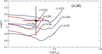
Figure 1. Illustration of the dependence of luminosity and temperature on progenitor mass M and mixing-length parameter α. Lines show the H-R diagram near the RSG for various MESA models labeled by (α, M). The dashed line shows the best-fit model.
Download figure:
Standard image High-resolution imageA grid of over 500 models were run as summarized in Table 6. These models were evaluated using a χ2 analysis. The first analysis was based on a comparison of the EG models with the adopted constraints on luminosity, radius, and surface temperature (ignoring mass loss). In this step χ2 was determined from the simultaneous goodness of fit to L, T and R. Hence, we write

where  is the point along the evolutionary track for each model that minimizes the χ2 and σi is the distance toward that point from the center to the surface of the three-dimensional error ellipse. The best fit from this calculation was found to be for masses in the range M =
  M⊙ and
  .
.
Figure 2 shows contours in the mass versus mixing-length parameter α plane. Contours indicate the 1σ (66%), 2σ (95%), and 3σ (99.7%) confidence limits. The models with progenitor masses from 14 to 30 M⊙ were run again using an adopted Reimers mass-loss rate, as described below. A mixing-length parameter α = 1.8–1.9 was chosen for these models, since α appears to have a shallow minimum around that value. We note, however, that only an upper limit to α could be determined, and we will argue below based on the observed surface convective velocities that a value of α = 1.4 ± 0.2 is preferred near the surface. Nevertheless, fitting the observed luminosity and temperature in particular requires a value of α ∼ 1.8–1.9 as illustrated in Figures 1 and 2.
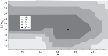
Figure 2. Contours of constant goodness of fit in the plane of progenitor mass M vs. mixing-length parameter α for EG models. The shaded regions indicate the 1σ (66%), 2σ (95%), and 3σ (99.7%) confidence limits as labeled.
Download figure:
Standard image High-resolution imageModels with mass loss were then evaluated again using both the EG code and the MESA codes in a χ2 analysis based on a comparison with not only the adopted luminosity, radius, and surface temperature but also the current adopted mass-loss rate  and the total ejected mass Mej. Since the mass-loss rate rises substantially as the models approach the base of the RGB, we integrate the ejected mass from that point to compare with the observed ejecta around the star. In these more constrained cases then χ2 is determined from

All of the evaluations found χ2 to be minimized for M = 20 M⊙. The best fits for both codes were for a progenitor mass of M =  . Figure 3 shows the comparison of the three χ2 analyses for χ2 versus mass based on the EG models. From this we deduce a best-fit (∼1σ C.L.) mass of
  for both codes and
  for the EG model, or
  with the MESA models. The slightly larger value for α with the MESA code is due to the slightly higher opacities that cause the models to expand more in the RSG phase and have slightly cooler surface temperature for a given α.

Figure 3. χ2 vs. progenitor mass M as evaluated by three different χ2 analyses. The black line shows the analysis for models evolved without mass loss and evaluated by comparing with observed luminosity, radius, and surface temperature. The gray lines show the analyses for models evolved with a Reimers mass-loss rate. The dark gray line represents the analysis with the comparison with observed luminosity, radius, surface temperature, and mass-loss rate, while the light gray line uses the same analysis but with total ejected mass as well. Notice how the minimum becomes better defined as more parameters are employed in the evaluation of χ2.
Download figure:
Standard image High-resolution imageFigure 4(a) shows the H-R diagram for the 20 M⊙ EG progenitor model with a Reimers mass-loss rate, while the solid line on Figure 4(b) shows the track generated by the MESA code. The tracks are nearly indistinguishable. The error ellipses from the adopted constraints on L and T are also shown. In both cases, the error ellipse encloses the track at the 1σ level. A summary of the "best-fit" parameters deduced in this study is given in Table 6, and the implied observed properties are given in Table 7. The mass loss of this model is consistent with the observed values, as we now discuss. For the best-fit models α Ori is currently on its ascent as an RSG, as expected, and has not yet ignited core carbon burning.

Figure 4. H-R diagrams for the best-fit models according to the χ2 analysis. Panel (a) is computed with the modified EG code. Panel (b) was computed with the MESA code. The dashed line in (b) shows the effect of convective overshoot with an overshoot parameter of f = 0.015. The error ellipse encloses the adopted uncertainty in T and L.
Download figure:
Standard image High-resolution imageTable 7. Summary of Fits to Observed Properties
| Parameter | Observed | EG | MESA |
|---|---|---|---|
| Age (106 yr) | ⋯ | 8.0 | 8.5 |
| M (M⊙) | ⋯ | 19.7 | 19.4 |
| Mej (M⊙) | 0.09 ± 0.05 | 0.09 | 0.09 |
 (10−6 M⊙ yr−1) (10−6 M⊙ yr−1) |
2 ± 1 | 2.0 | 2.0 |
 |
5.10 ± 0.22 | 4.97 | 4.99 |
| Teff (K) | 3500 ± 200 | 3630 | 3550 |
| R (R⊙) | 887 ± 203 | 774 | 821 |
 |
−0.5 | −0.05 | −0.010 |
 |
 |
39 | 42 |
| X(12C) (10−3) | 1.85 ± 0.80 | 2.6 | 3.0 |
| X(13C) (10−3) | 0.31 ± 0.20 | 0.13 | ⋯ |
| X(14N) (10−3) | 4.1 ± 1.1 | 2.3 | 3.7 |
| X(15N) (10−3) | ⋯ | 0.0022 | ⋯ |
| X(16O) (10−3) | 6.6 ± 2.0 | 8.9 | 9.9 |
| X(17O) (10−3) | 0.013 ± 0.006 | 0.0025 | ⋯ |
| X(18O) (10−3) | 0.011 ± 0.004 | 0.0019 | ⋯ |
Download table as: ASCIITypeset image
Note that our conclusion that a nonrotating star of around 20 M⊙ best fits the observations is consistent with the models of Meynet et al. (2013). In that paper it was also noted, however, that adding rotation causes tracks to be more luminous for a given initial mass. For example, in a rotating model with an initial rotation with  , the current observed properties are best fit with a progenitor mass of around 15 M⊙. This, however, corresponds to a rather high progenitor rotation rate. The quantity vcrit is the maximum equatorial rotational velocity such that the centrifugal force is exactly balanced by gravity.
We also note that our best-fit nonrotating mass and radius imply  and
and  (R⊙/M⊙). This value of surface gravity is larger than the value log g = −0.5 determined in the model atmospheres of Lobel & Dupree (2000). The ratio R/M is similarly a factor of two smaller than the value
  determined in the limb-darkening model of Neilson et al. (2012). If we allow for the fact that the model fits to stellar radius and mass are uncertain by about 25% owing to the uncertainties in the observed properties, then much of this discrepancy could be explained if the mass were near the lower range and the radius near the upper range of the uncertainty. Just varying the mass alone with the observed radius would require
  M⊙, as pointed out in Neilson et al. (2012).
Two remarks regarding these discrepancies are in order. One is that these estimates are for the current mass of Betelgeuse and not the initial mass. Possibly this suggests an earlier epoch of much more vigorous mass loss. For example, the mass estimate of Neilson et al. (2012) is consistent with the large mass loss in the rapidly rotating models of Meynet et al. (2013). Another possibility is that a larger radius could also resolve these discrepancies. This might, for example, be due to the observed rather clumpy extended surface of this star (e.g., Chiavassa et al. 2011; Kervella et al. 2011), i.e., the effective limb-darkening radius might be larger than the spherical photospheric radius of the models.
3.1. Convective Overshoot
We utilize a standard mixing-length theory treatment for convection. The Ledoux criterion (i.e., including chemical inhomogeneities) is utilized to identify convective instabilities, and semiconvection is also included (i.e., mixing in regions that are Schwarzschild unstable though Ledoux stable) as described in the MESA code (Paxton et al. (2013).
In a fully three-dimensional hydrodynamical treatment of convection there can be hydrodynamical mixing instabilities at convective boundaries. This is called convective overshoot. As we shall see below, the outer region of Betelgeuse consists of a rapidly developing convective envelope extending deep into the star. There is also convection in the central helium-burning core. Because of this outer convective envelope, the observed properties of this star can be sensitive to the subtitles of convective overshoot at the boundary of the hydrogen-burning shell. Hence, we have also made a study of the affects of convective overshoot on the models derived here.
In both codes this is accomplished via extra diffusive mixing at the boundaries of convective regions. In the MESA code (Paxton et al. 2011, 2013) convective overshoot is parameterized according to the prescription of Herwig (2000). That is, the MESA code sets an overshoot mixing diffusion coefficient

where DMLT is a diffusion coefficient derived from mixing-length theory and  is the pressure scale height. The free parameter f denotes the fraction of the pressure scale height that extends a distance z into the radiative region. A typical value for f for AGB stars is f ≈ 0.015 (Herwig 2000), with a maximum value consistent with observed giants of f < 0.3. We consider this range in the models.
However, as we shall see, although the addition of convective overshoot affects the location of the main-sequence turnoff, it has very little effect on the giant branch. Hence, the observed temperature and luminosity cannot be used to fix the convective overshoot parameter. As we discuss below, however, the observed surface abundances place a constraint on the mixing parameter f. Also as discussed below, the age of this star is slightly decreased when convective overshoot is added. Presumably this is due to changes in thermonuclear burning as material is mixed into radiative zones.
3.2. Mass Loss
The total ejected mass since arriving at the base of the RGB is a small fraction of the total mass both observationally and in the best-fit models. The mass-loss rate increases considerably as the track approaches the base of the RGB. Therefore, to better identify the location of this star along its track, we can compare the observed accumulated ejected mass along with various integrated mass-loss rates since arriving at the base RGB. We note, however, that the mass loss begins slightly earlier in rotating models (Meynet et al. 2013).
As shown in Table 5, our adopted current observed mass-loss rate is (2 ± 1) × 10−6M⊙ yr−1 with a total ejected mass of 0.09 ± 0.05 M⊙ (Knapp & Morris 1985; Glassgold & Huggins 1986; Bowers & Knapp 1987; Skinner & Whitmore 1987; Mauron 1990; Marshall et al. 1992; Young et al. 1993; Huggins et al. 1994; Mauron & Guilain 1995; Guilain & Mauron 1996; Harper et al. 2001; Plez & Lambert 2002; Ryde et al. 2006; Le Bertre et al. 2012; Humphreys 2013; Richards 2013).
This would correspond to a lifetime of roughly between 3 × 10⁴ and 7 × 10⁴ yr in the RSG phase. However, one expects that the mass-loss rate would have varied during the initial ascent from the base of the RGB. Hence, we have considered the various mass-loss rates given below to integrate the total ejected mass from the stellar models.
Realistically modeling the mass loss from Betelgeuse would be quite complicated. It appears to be episodic (Humphreys 2013) and likely involves coupling with the magnetic field (Thirumalai & Heyl 2012), as well as the normal radiatively driven wind. Indeed, there is evidence of a complex MHD bow shock around this star (Mackey et al. 2012, 2013; Mohamed et al. 2012, 2013). Nevertheless, for comparison of observations with models we have considered various parameterized mass-loss rates (Reimers 1975, 1977; Lamers 1981; Nieuwenhuijzen & de Jager 1990; Feast 1992; Salasnich et al. 1999). For the Reimers (1975) rate,

where L, R, and g are in solar units. The observed rate requires a mass-loss parameter of η = 1.34 ± 1 for a ∼20 M⊙ star of the adopted L and R. This value is not atypical for giants and is very close to the value inferred by Le Bertre et al. (2012). The Reimers (1977) rate

implies a mass-loss rate of 3.32 × 10⁻⁶M⊙ yr−1, which is again consistent with observed rates and the Reimers (1975) value. On the other hand, the Lamers (1981) rate
gives a present mass loss of 8.80 × 10⁻⁶ M⊙ yr−1, which is higher by a factor of ∼4 than the adopted current mass ejection rate. The mass-loss rate of de Jager et al. (1988)

would predict a mass-loss rate of 8.40 × 10⁻⁶M⊙ yr−1, which is also higher by a factor of ∼4 relative to our adopted rate. The rate from Salasnich et al. (1999)

predicts a mass-loss rate of 2.98 × 10⁻⁵M⊙ yr−1, which is based on the mass-loss pulsation–period relation of Feast (1992)

This implies a very high current mass-loss rate of 1.96 × 10⁻⁵M⊙ yr−1 (using the observed 420-day pulsation period).
Based on this comparison, we adopt the Reimers (1975) rate with  as best representing this star. We note, however, that this total mass loss may only be a lower limit to the ejected mass along the RSG phase. This is because not all of the ejected mass may be currently detectable if it was ejected sufficiently far in the past.
3.3. H-R Diagram
Figures 4(a) and (b) show H-R diagrams for the 20 M⊙ modified EG model and the MESA-code model, respectively. The H-R diagrams are quite similar. The dashed line in panel (b) of Figure 4 shows the H-R diagram for a 20 M⊙ model calculated with the MESA code with an overshoot parameter f = 0.015. Here one can see that the main effect of the convective overshoot is to increase the luminosity of the main-sequence turnoff and the base of the RGB. It does not, however, affect the luminosity or temperature of the star as it moves up the giant branch. Hence, there is little constraint on convective overshoot from the observed luminosity and temperature. A value of f = 0.3, however, moves luminosity of the base of the RGB all the way up to the observed luminosity. This much overshoot, however, is inconsistent with the observed C and N abundances, as we shall see below.
In both of our best-fit models, the first dredge-up occurs shortly after reaching the base of the RGB. This is when the surface nitrogen is enriched. This means that only models in which the current temperature and luminosity correspond to the ascent up the RSG phase can be consistent with this star.
3.4. Best-fit Model for the Present Star
In spite of the large uncertainties, the adopted mass-loss rate and ejected mass around this star can limit the possible present location of this star along its evolutionary track if we accept that the star has only recently ascended the RSG phase as the best-fit models imply. Hence, we (somewhat arbitrarily) deduce the current age of the star from the amount of mass ejected from the base of the RGB. We checked, however, and the deduced age and properties do not depend on this assumption.
Figure 5 shows a comparison of the total mass ejected as a function of time from the base of the RGB. These curves are based on the Reimers (1975) rate with a mass-loss parameter of η = 1.34 for both the EG (thick solid line) and the MESA (thick dashed line) 20 M⊙ progenitor models. With our adopted parameters we find that by the time the star reached the main-sequence turnoff it had lost 0.1 M⊙ in both models, and by the time it reached the base of the RGB it had lost 0.3–0.4 M⊙. It is possible, however, that our adopted Reimer's mass-loss parameter overestimates the main-sequence mass loss. Winds during the main-sequence phase are very different from the winds during the RSG phase. During the main sequence, winds are mainly radiatively driven, while the RSG winds involve molecules, dust, etc. Hence, these tracks represent upper and lower limits for the mass-loss evolution of this star.

Figure 5. Thick solid line shows the total ejected mass Mej (in M⊙) for the best-fit 20 M⊙ progenitor model from the modified EG code as a function of time. The thick dashed line is from the MESA model. The dot-dashed line is for the MESA model with an overshoot parameter of f = 0.015. Shaded regions indicate the areas excluded by the adopted limits on the total ejected mass.
Download figure:
Standard image High-resolution imageThe shaded areas indicate the excluded regions based on our adopted uncertainty on the total ejected mass in Table 5. The MESA track indicates a more advanced lifetime as it ascends the RGB. The older age for the MESA models is mostly attributable to the increased opacity at low densities and temperatures in the MESA model. This leads to lower luminosity and hence longer lifetimes. In the context of these models, the amount of mass ejected corresponds to a present age since the zero-age main sequence (ZAMS) of ∼8.0 Myr in the EG model and about 8.5 Myr in the MESA model. For both models the ages are about 0.1 Myr less when convective overshoot is included. Here we adopt the ages in the MESA model without convective overshoot as the most realistic, but we include the EG model results as an illustration of the uncertainty in this age estimate.
3.4.1. Interior
Based on our estimated location in its ascent up the RSG phase, we now examine the interior structure associated with this point in its evolution. Figure 6 summarizes some of the interior thermodynamic properties. The EG and MESA models give almost identical results for the interior thermodynamic properties. In both models the star is characterized at the present time by the presence of a developing carbon–oxygen core up to the bottom of the outer helium core at ∼3–4 M⊙.

Figure 6. Thermodynamic state variables ρ, T, and P as a function of mass for our best-fit 20 M⊙ model.
Download figure:
Standard image High-resolution imageThe central density has risen to ∼103 g cm−3 with a central temperature of ∼108 K. Outside of the developing C/O core there is a region of steadily decreasing density in the outer helium core and hydrogen-burning shell that extends to the outer envelope consisting of low-density (∼10−6 g cm−3) material. The outer envelope reaches to 90% of the mass coordinate of the star. This is followed by rapidly declining density and the development of an outer surface convective zone.
The best-fit MESA model left the main sequence about 106 yr ago, while for the EG model it was only about 3 × 10⁵ yr ago. Both models reached the base of the RGB about 40,000 yr ago. We followed the star through the final exhaustion of core helium burning in both codes, followed by brief epochs of core carbon, neon, oxygen, and silicon burning until core collapse and supernova at an age of 8.5 Myr since the ZAMS for the MESA code. Our best guess is that the star will supernova in less than ∼100,000 yr (even longer in the EG model). We note, however, that the error ellipse encompasses the entire track, so that the star could be further along in its evolution. The constraint that it has passed the first dredge-up, however, means that the star is ascending the RSG phase. Our result is based on mass loss from the base of the RGB and is therefore a lower limit to how far it has evolved as an RSG.
3.4.2. Composition
Figures 7(a)–(b) show composite plots of isotopic abundances versus interior mass from the best-fit EG and MESA 20 M⊙ progenitor models. These are compared with the surface isotopic compositions determined by Harris & Lambert (1984) and Lambert et al. (1984). The surface CNO surface abundances computed in both models are quite consistent with the observations as shown by the points in the figures. Hence, the models have correctly evolved the star through the first dredge-up.

Figure 7. Composite interior abundances as a function of interior mass for the best-fit 20 M⊙ progenitor EG (top panel) and MESA (bottom panel) models. Points are surface abundances from Table 4.
Download figure:
Standard image High-resolution imageThe present-day interior compositions were similar for the two models except that the interior carbon core is slightly larger in the MESA models owing to the slightly older lifetime. Also, the convective core seems to be less efficiently mixed in the EG model than in the MESA simulation. We attribute this to the more sophisticated mixing treatment in the MESA code (Paxton et al. 2013). Nevertheless, in both models the C/O core has built up to a mass fraction of 40%–50% C and O and extends to about 3 M⊙. Above this, the He core extends to about 6 M⊙, while the bottom of the outer convective envelope is at 8 M⊙ in the EG model but has already descended to ∼10 M⊙ in the MESA model.
3.5. Convection and Convective Overshoot
The interior convective properties of the EG and MESA models were quite similar. Figure 8 shows a Kippenhahn diagram of the convective regions over the lifetime of a star for a 20 M⊙ model with α = 1.8 and a convective overshoot parameter of f = 0.015. An arrow at the bottom indicates our deduced present age for Betelgeuse. Dark shaded regions are unstable to convection by the Ledoux criterion. Lighter regions indicate the range of convective overshoot. One can see from this that the star currently has a rapidly developing outer convective envelope extending deep into the interior. One can also see the recent onset of mass loss for this star.
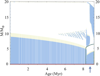
Figure 8. Kippenhahn diagram showing evolution of convective zones for a 20 M⊙ model computed with the MESA code with α = 1.8 and a convective overshoot parameter of f = 0.015. Darker shading indicates regions that are unstable to convection by the Ledoux criterion. Lighter shading indicates the regions of convective overshoot.
Download figure:
Standard image High-resolution imageThe observed surface abundances, however, can be used to place constraints on convective overshoot at the base of the outer convective envelope. The three panels of Figure 9 illustrate the effects of adding convective overshoot with f = 0.015 to the models. One can see that the main effect of convective overshoot is to extend the bottom of the outer convective envelope from 10 to 12 M⊙. It also causes the surface abundances of C, N, and O to shift away from agreement, with the biggest discrepancy for 14N, which changes from agreement to a 3σ discrepancy. The reason for these discrepancies is that convective overshoot tends to minimize the influence of the first dredge-up. Based on this, we conclude that the overshoot parameter for the outer region is constrained to be f < 0.10 at the 2σ confidence level and is most consistent with f = 0.0. Hence, we adopt f = 0.0 for our best-fit models. We note, however, that this constraint is not necessarily valid for the inner convective core, where convection could behave quite differently (e.g., Viallet et al. 2015).
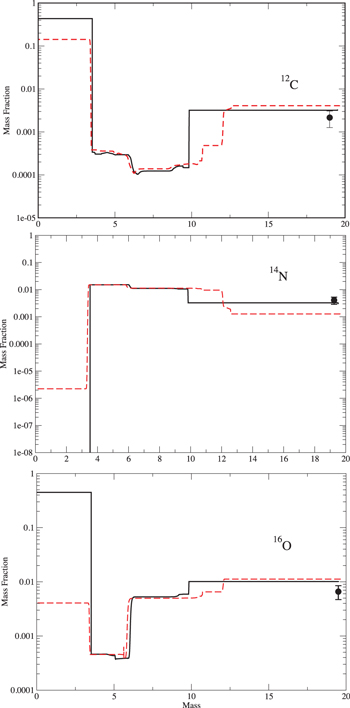
Figure 9. Effects of convective overshoot on elemental composition. Solid line shows interior C (top panel), N (middle panel), and O (bottom panel) abundances as a function of interior mass for the 20 M⊙ progenitor MESA model. Points are total elemental surface abundances from Table 4. Dashed lines shows the effect of convective overshoot with mixing parameter f = 0.015.
Download figure:
Standard image High-resolution image3.6. Hot Spots and Convection
It has been suggested (Buscher et al. 1990; Wilson et al. 1997; Freytag et al. 2002; Montargés et al. 2015) that the occurrence of bright spots on the surface of Betelgeuse is the result of convective upwelling material at higher temperature. It is possible to examine whether the occurrence of such features is consistent with simple mixing-length theory in our stellar evolution models. That is, the distance lc over which a surface convective cell moves is characterized in mixing-length theory by the pressure scale height:

The condition for which a convective cell reaches the photosphere is

where r is the region from which the convective cell begins its upward motion. The temperature Ths at which this cell appears on the surface as a hot spot is then given by

where the adiabatic temperature gradient is
The change in luminosity due to the occurrence of such a spot is then
where we have assumed that lc also characterizes the size of a convective cell when it reaches the surface. This seems justified by 3D simulations and images (Freytag et al. 2002; Chiavassa et al. 2012; Kervella et al. 2013b) that exhibit convective-cell profiles that are roughly spherical. Indeed, a number of detailed three-dimensional numerical simulations of deep convective envelopes have confirmed the adequacy of mixing-length theory except near the interior boundary layers (Chan & Sofia 1987; Cattaneo et al. 1991; Kim et al. 1996). In particular, they also show approximately constant upward and downward mean velocities (Chan & Sofia 1986), implying a high degree of coherence of the giant cells.
In Buscher et al. (1990) a single bright feature was detected that contributed ∼10%–15% of the total observed flux. In Wilson et al. (1997) the observations were consistent with at least three bright spots contributing a total of 20% to the total luminosity. In their best-fit model the hot spots were taken to have a Gaussian FWHM of 12.5 mas corresponding to as much as one-third of the total surface area or about 10% of the surface per hot spot. Haubois et al. (2009) observed two hot spots attributing to about 10% of the total luminosity. In Freytag et al. (2002), the best fit for their radiation hydrodynamic model has luminosity variations of no more than 30% for the total luminosity, with numerous upwelling hot spots. While their model supports the hot spot theory and most parameters fit the data, they derive a mass of only 5–6 M⊙, which is inconsistent with the observed luminosity and temperature for this star. Further work by Dorch (2004) using MHD modeling may improve on this inconsistency. Here we point out that a simple mixing-length model is marginally adequate to explain the observed hot spots, as we now describe.
Figure 10 shows the surface convection condition,  , as a function of interior radius for a 20 M⊙ model with convective overshoot and α = 1.8. This shows that the typical size of a convective cell near the surface is less than about 2% of the radius of the star. Hence, the observed surface hot spots that cover as much as ∼10% of the stellar disk would have to result from large fluctuations in the size distribution. The temperature change at the surface from our model is ΔT ≈ 300 K, which for a large fluctuation in spot size would correspond to a 20% change in luminosity and be consistent with the observations.
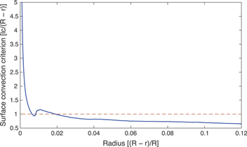
Figure 10. Surface convection criterion  as a function of radius near the stellar surface for a 20 M⊙ model computed with the MESA code.
Download figure:
Standard image High-resolution imageWe can also deduce a convective velocity by equating the work done in moving the convective cells to the kinetic energy in the bubbles:

where  denotes the difference between the temperature gradient in the convective cell and that in the surroundings, α is the mixing-length parameter, and β = 1/2 because we are measuring at the center of the convective cell. We calculate a convective velocity at the surface of
  km s−1. Lobel & Dupree (2001) deduced a value of
  km s−1. The convective velocity has a dependence on α and can therefore serve as a constraint on α. The best-fit models had α = 1.8–1.9. However, using the value of vc derived from Lobel & Dupree (2001) and Lobel (2003a, 2003b) would imply that α = 1.4 ± 0.2 near the surface.
An alternate explanation posed by Uitenbroek et al. (1998) suggests that the hot spots result from shock waves caused by pulsations of the stellar envelope. They use Bowen's (1988) density stratification model calculated by Asida & Tuchman (1995). In this model, the stellar envelope pulsates, causing repetitive shock waves that create a density profile that is shallow with respect to the density predicted by hydrostatic equilibrium. Future numerical work should be done to resolve which of the two scenarios is correct for α Orionis.
3.7. Periodic Variability
In addition to the random variability due to upwelling convective hot spots, one also expects Betelgeuse to exhibit regular pulsations. As a massive star ascending the red giant, one expects α Ori to exhibit the regular radial pulsations associated with a long-period variable star. Indeed, Betelgeuse is classified (Samus et al. 2011) as a semiregular variable with an SRC subclassification and a period of 2335 days (6.39 yr). Analyzing the periodicity of this star is difficult, however, as more than one cycle appears to be operating simultaneously and intermittently. In Dupree et al. (1987) and Smith et al. (1989) a pulsational period of 420 days was detected that subsequently disappeared. In Dempsey (2015) a pulsation period of 376 days was deduced using data in the AAVSO database.
It is worthwhile to analyze the implied periodicity from the best-fit model deduced here. Although a detailed model is beyond the scope of the present paper, we can estimate the period to be expected from a one-zone linear adiabatic wave analysis of radial oscillations (Cox & Giuli 1968). For a surface shell on the exterior of a homogeneous star of radius R and mass M and a surface adiabatic equation-of-state index γ, the pulsation period Π is just given by a linearization of surface hydrodynamic equations of motion for a radial perturbation δR,

which has a solution of simple harmonic motion corresponding to a period of
where  is the mean density of the star. For our best-fit model the mean density is
  g cm−3 and the mean adiabatic index is
  . This implies a pulsation period of
  s. This seems reasonably close to the intermittent 420-day pulsation period, particularly given the simplicity of the model and the fact that the observed period may be influenced by higher modes. Clearly, a more detailed nonlinear, nonadiabatic analysis that would also determine the amplitude of the pulsations is warranted.
We attempted a more realistic radial pulsation calculation for our model of α Orionis using both the pulsation code from Hansen & Kawaler (1994) and the one in the MESA code. Although the calculated periods for certain harmonics agree with the observed periodicity of α Orionis, the fundamental mode and first overtone could not be modeled well. This problem may be resolved by considering nonadiabatic pulsations coupled to the convection (Xiong et al. 1998). Results of 3D simulations of RSG stars (Jacobs et al. 1998; Freytag et al. 2002) and Betelgeuse in particular (Chiavassa et al. 2011; Freytag & Chiavassa 2013) confirm the development of large-scale granular convection that generates hot spots. Such convective motion should also drive pulsations and should be analyzed in detail to explain the different pulsation frequencies for α Orionis. Indeed, such large-scale convective motion may also contribute to the secondary periods of this star (Stothers 2010).
4. ORIGIN
Based on our inferred present age for this star, one can deduce the past positions of α Orionis using the Hipparcos measured proper motion of  mas yr−1 and
  mas yr−1 (Harper et al. 2008), combined with the measured radial velocity of 21.0 ± 0.9 km s−1 (Wilson 1953). The galactic coordinates for α Ori are (X, Y, Z) = (−121.8, −43.8, −20.4) and (U, V, W) = (21.4, −10.2, 14.6). Traced back 10 Myr, this gives (X, Y, Z) = (−339, 59.9, −163.4).
The Orion OB 1a association has been considered a candidate for the origin of α Orionis. The association's age is ∼10 Myr (Brown et al. 1994; Briceño et al. 2005), comparable with our predicted age for α Orionis of ∼8.5 Myr. The distance to the Orion OB 1a association is currently 336 ± 16 pc, measured using the mean distances to the subgroups (Brown et al. 1999). However, the association is moving mainly radially ∼28 km s−1 with negligible detected proper motion (Brown et al. 1999; de Zeerw et al. 1999). This motion traced back 10 Myr gives a change in position of only ∼290 pc and is consistent with the implied location of α Orionis at birth. Recently, however, Bouy & Alves (2015) have discovered a new OB association that may be the origin of Betelgeuse. Nevertheless, one can conclude that α Orionis most likely did originate in the Orion Nebula. These results agree with a similar analysis done by Wing & Guinan (1998).
The age of α Ori also corresponds well with the age of the Sco-Cen subgroups. However, the position of α Orionis 10 Myr ago is over 500 pc away from the position of the Sco-Cen cloud as determined by Mamajek et al. (2000).
5. FUTURE SUPERNOVA
As for the future, α Orionis will continue burning He. Eventually core C burning will begin, followed by core O burning and then core Si burning as it continues to increase in luminosity. We estimate that in a little less than 105 yr, α Orionis will supernova as a Type IIp, releasing 2.0 × 1053 erg in neutrinos along with 2.0 × 1051 erg in explosion kinetic energy (Smartt 2009) and leaving behind a neutron star of mass ∼1.5 M⊙. Figure 11 shows the interior density and temperature profile for this star just prior to collapse. At this point the star has evolved to an ∼1.5 M⊙ Si, Fe core and is about to collapse.

Figure 11. Interior temperature vs. density plot near the end of the lifetime of the best-fit 20 M⊙ progenitor model obtained with the MESA code.
Download figure:
Standard image High-resolution image
When this supernova explodes, it will be closer than any known supernova observed to date, and about 19 times closer than Kepler's supernova. Assuming that it explodes as an average SN II, the optical luminosity will be approximately −12.4, becoming brighter than the full moon. The X-ray and γ-ray luminosities may be considerable, though not enough to penetrate the Earth's atmosphere.
The interaction of such a supernova shock with the heliosphere has been studied in detail in Fields et al. (2008). In that study it was demonstrated that unless a typical supernova occurs within a distance of 10 pc, the bow-shock compression of the heliosphere occurs at a distance beyond 1 AU. Hence, for the adopted distance of 197 pc, the passing supernova remnant shock is not likely to directly deposit material on Earth. Nevertheless, we can surmise some of the properties of the passing shock based on a spherically symmetric Sedov–Taylor solution (Landau & Lifshitz 1987; Fields et al. 2008). The time for the arrival of the supernova shock front will be
where the numerical factor β = 1.1517 for an adiabatic index of γ = 5/3, mp is the hydrogen mass, nISM is the ambient interstellar medium density, ESN is the supernova explosion energy, and RSN is the distance to the supernova. For our adopted distance of 197 pc and explosion energy of 2 × 1051 erg, we would expect the shock to arrive in about 6 × 10⁶ yr. The timescale for the passage of this supernova shock will be >1 kyr. As the shock arrives, its velocity will have diminished to

while the speed of the shocked material flowing behind the shock will be

The density of material behind the supernova shock will be  , while the total sum of ram pressure and thermal pressure behind the shock will be
This is to be compared with the pressure of the solar wind for which

A stagnation point will develop at the distance Rstag at which the two pressures are equal, giving

which for our adopted distance and energy implies  , well beyond Earth.
6. CONCLUSIONS
We have deduced quasi-static spherical models for α Orionis constrained by currently known observable properties. Table 7 summarizes a comparison of the observable properties of this star with those from the best-fit EG and MESA models. One can see that, for the most part, the models reproduce the observed properties. The fits to observations are optimized for a 20 M⊙ progenitor that is ascending the RSG phase and has passed through the first dredge-up phase near the base of the RGB. It currently has a rapidly developing outer convective envelope.
A notable exception, however, to the agreement between predicted and observed properties is the surface gravity. As discussed above, a surface gravity of  was deduced from the model atmospheres of Lobel & Dupree (2000). There is a discrepancy of −0.4 dex between that value and the value deduced from the best-fit models. Since g scales as
  , it is most sensitive to the radius, and this discrepancy could be resolved if the effective radius of the surface gravity is much larger than the observed angular diameter. The other possibility is that this star has undergone substantial mass loss, perhaps owing to rapid rotation (Meynet et al. 2013).
The mass loss, surface and core temperatures, and luminosity are consistent with this star having relatively recently begun core helium burning. As such, our best model is most consistent with a mixing-length parameter of α = 1.8–1.9 and a present age of t = 8.5 Myr. The size and temperature of the convective up-flows are consistent with observed intermittent hot spots only if such spots correspond to large fluctuations in the typical surface convective cell size, and they are probably due to more complicated MHD evolution near the surface. Also, the surface turbulent velocity seems to require a smaller mixing-length parameter of α ∼ 1.4 near the surface. The observed light-curve variability is consistent with the derived mean density and equation of state for this star. We estimate that this star will begin core carbon burning in less than ∼105 yr and will supernova shortly thereafter. Although the supernova shock will arrive about 6 × 10⁶ yr after the explosion, it is not expected that the supernova debris will penetrate the heliosphere closer than about 2.5 AU.
What is perhaps most needed now are good multidimensional turbulent models together with a nonlinear pulsation treatment to further probe the variability of this intriguing star during its current interesting phase of evolution.
Work at Notre Dame is supported by DoE Nuclear Theory grant number DE-FG02-95ER40934. One of the authors (N.Q.L.) acknowledges support from the NSF Joint Institute for Nuclear Astrophysics.