How Can Remote Sensing Help Monitor Tropical Moist Forest Degradation?—A Systematic Review


TERRA Teaching and Research Centre (Forest is Life), Gembloux Agro-Bio Tech, University of Liege, Passage des Déportés n°2 5030 Gembloux, Belgium
*
Author to whom correspondence should be addressed.
Remote Sens. 2020, 12(7), 1087; https://doi.org/10.3390/rs12071087
Submission received: 4 March 2020 / Revised: 25 March 2020 / Accepted: 26 March 2020 / Published: 28 March 2020
(This article belongs to the Special Issue Forest Degradation Monitoring)
Abstract
:
In the context of the climate and biodiversity crisis facing our planet, tropical forests playing a key role in global carbon flux and containing over half of Earth’s species are important to preserve. They are today threatened by deforestation but also by forest degradation, which is more difficult to study. Here, we performed a systematic review of studies on moist tropical forest degradation using remote sensing and fitting indicators of forest resilience to perturbations. Geographical repartition, spatial extent and temporal evolution were analyzed. Indicators of compositional, structural and regeneration criteria were noted as well as remote sensing indices and metrics used. Tropical moist forest degradation is not extensively studied especially in the Congo basin and in southeast Asia. Forest structure (i.e., canopy gaps, fragmentation and biomass) is the most widely and easily measured criteria with remote sensing, while composition and regeneration are more difficult to characterize. Mixing LiDAR/Radar and optical data shows good potential as well as very high-resolution satellite data. The awaited GEDI and BIOMASS satellites data will fill the actual gap to a large extent and provide accurate structural information. LiDAR and unmanned aerial vehicles (UAVs) form a good bridge between field and satellite data. While the performance of the LiDAR is no longer to be demonstrated, particular attention should be brought to the UAV that shows great potential and could be more easily used by local communities and stakeholders.
1. Introduction
1.1. Threats to Tropical Moist Forests
While unprecedented climate change is taking place on a global scale, mainly caused by human carbon emissions [1], and while the great majority of indicators of ecosystems and biodiversity are showing a rapid decline because of human drivers [2,3], forests are important to preserve. In particular, tropical forests that contain over half of Earth’s species [4] and are among the terrestrial biomes with the largest flows of ecosystem services [5], on which billions of people depend [6]. Tropical forests also play a key role in global carbon flux by accounting for ~70% of the gross C sink in the world forests [7,8]. Yet, tropical forests are experiencing significant degradation [9], defaunation and deforestation [3,7,10], mainly caused by human activities [2]. Even if tropical forest loss is responsible for significant carbon emissions [11,12], these forests are today still considered as a carbon sink [7,13]. However, this trend could not continue over the next decades because carbon sink saturation will appear in tropical forests, firstly in the Amazon and secondly in Africa [13].
On a global scale, the decreasing of forests area only occurs in tropical regions [14], especially in tropical moist forests where 84 000 km² have been lost between 1982 and 2016 [15]. While more forests are under protection, Intact Forest Landscape (IFL), which is a “seamless mosaic of forest and naturally treeless ecosystems with no remotely detected signs of human activity and a minimum area of 500 km²”, and primary forests are still impacted by these changes [16,17]. The degradation of forests also covers significant areas with 20%, 63% and 65% that are considered as second growth forests after human activities, respectively in the Amazon Basin, Southeast Asia and Congo Basin [18]. Consequences are significant: biodiversity loss [19,20], soil degradation [21,22], negative impact on economic activities and households products [23,24], spread of diseases [25] and carbon emissions [7,26]. In tropical moist forests regions, drivers of forest degradation are timber logging, human-made fires, fuel-wood collection, small scale agriculture and mining activities [9,27,28]. In Central Africa, deforestation and degradation are linked to population density and agricultural activities, as well as access to resources, including mining, which promotes urbanization [10].
To mitigate climate change and biodiversity loss, and to stop degradation and deforestation processes, action must be taken at all levels—people, local, global—by all countries—poor, middle-income, rich—and in the same direction. Recently, the United Nations (UN) called to all sectors of society to mobilize for a decade of action with the aim to deliver 17 sustainable development goals by 2030. In particular, the 15th objective aims to ensure the conservation, restoration and sustainable use of forests [29]. Since 2008, the UN-REDD Programme (United Nations Reducing Emissions from Deforestation and Degradation Programme), set up under the United Nations Framework Convention on Climate Change (UNFCCC), promotes developing countries to protect their environment by adding value to the carbon stored in forests [30]. These objectives require the ability to localize, measure and monitor forest change and to define the two main causes of these changes: forest degradation and deforestation. Especially for the UN-REDD Programme, there is a need for a robust, transparent, consistent and accurate Measurement, Reporting and Verification (MRV) system to operate effectively [30,31].
1.2. Define and Measure Forest Degradation
While deforestation is the transformation from forest to non-forest area, over 50 definitions related to forest degradation were recently reported in peer-reviewed literature [32]. The IPCC (Intergovernmental Panel on Climate Change) defines forest degradation as “direct human-induced long-term loss (persisting for X years or more) of at least Y% of forest carbon stocks [and forest values] since time T and not qualifying as deforestation or an elected activity under Article 3.4 of the Kyoto Protocol” [33]. This definition only focuses on carbon stocks and depends on the individual country. This is also what the FAO (Food and Agriculture Organization of the United Nations) supports by letting countries define the term "degraded forest" [34]. The general definition of forest degradation refers to the reduction of the capacity of a forest to produce goods and services [35]. This definition leads to many interpretations and is linked to human benefits, meaning that if there is forest perturbation that does not impact humans, it will not be considered as forest degradation. This anthropocentric vision needs to be complemented by an approach that takes into account broader ecological processes regardless of their potential link with human societies such as forest dynamics and resilience [36,37]. Ecosystem resilience can be defined as the ability to recover the structure and function of its reference state after a disturbance and without external intervention [38]. While resilience and degradation are usually separately considered, they can be mixed by interpreting forest degradation through the frame of ecological resilience, and with reference to forest dynamics [36,37]. A degraded forest can be thus defined as “a state of anthropogenically induced arrested succession, where ecological processes that underlie forest dynamics are diminished or severely constrained”[36]. Whereas, degradation is a temporal process before the “degraded state” during which forests attributes decline (Figure 1). Indicators of forest degradation should reflect this ecological process. When a forest is resilient, these indicators can recover the reference state after disturbance, but the recovery takes more time if disturbances are more intense and/or more frequent. The forest is losing resilience and so, is being degraded until a tipping point, at which the forest has reached the degraded state and cannot recover by itself.
Studying forest degradation through the frame of resilience involves defining reference states, indicators of resilience and benchmarks by which the forest is considered as degraded (Figure 1). The degradation process (upper part of Figure 1) can also be more accurately defined by measuring disturbances intensity and frequency. In the literature, reference state definitions and indicators of resilience vary following author and study objectives [36,37,38]. Degradation benchmarks are not well known as they involve having reached a point of no return for a specific ecosystem [37]. In light of these observations, compositional, structural and regeneration criteria can be analyzed to identify whether or not a forest is being degraded or is degraded [37]. Structure (e.g., canopy cover, diametric structure, biomass) and composition (e.g., specific richness, dominance of secondary species, presence of invasive species) give information about the forest state at a time. Studying forest degradation through the frame of resilience involves studying the phenomenon over time. Characterizing regeneration of a forest after disturbance (e.g., presence of shrubs, tree species or adult seed trees) can give information about forest future and its capacity to recover. For example, in the case of selective logging, forest composition can be altered: commercial species decrease while secondary species in logging gaps increase. Selective logging also induces changes in forest structure: loss in biomass, decrease of forest stands height and the emergence of canopy gaps. Regeneration after logging does not allow for restoring the initial forest composition: commercial species decline [39] and enrichment planting is needed to maintain them [40]. However, the biomass can recover quickly after disturbance [39,41]. It is so important to consider all three criteria (composition, structure, regeneration) to define whether a forest is degraded or not. Even though the regeneration of biomass suggests that the forest is resilient, it is not as if the initial composition cannot be restored without external interventions.
1.3. Remote Sensing to Measure Tropical Forest Degradation
Some documents are a good starting point to operationalize the definition of degraded forest in accordance with the IPCC guidelines [33,44]: the GOFC-GOLD (Global Observation of Forest and Land Cover Dynamics) sourcebook [45] and the methods and guidance from the GFOI (Global Forest Observations Initiative) [46] that focus on greenhouse gas emissions and carbon stocks variation in forests. Broader approaches consider several criteria together e.g., the production, the biodiversity, unusual disturbances, the protective function and the carbon storage of a forest [42]. Looking at degradation defined as a loss of resilience, adequate indicators of forest composition, structure and regeneration, as described in the previous section, need to be found [37]. Indicators requiring field data collection are time-consuming and logistically difficult to obtain. Especially in tropical moist forests that cover large areas, such indicators are difficult to access and are structurally complex. Remote sensing tools provide opportunities to more easily measure and spatialize indicators [47].
While deforestation is well detected on a global scale using different sensors and approaches, principally based on earth observation satellites [48], forest degradation, that appears at a smaller spatial and temporal extent, is more difficult to detect and to quantify. In recent reviews [49,50], different sensors (SAR, optical, LiDAR), image resolutions, spatial and temporal extents as well as indicators of degradation have been identified. Satellite data is the most used and improvement in mapping degradation should appear in the next few years by mixing SAR and optical data and by using very high-resolution data. SAR and LiDAR provide key information on forest structure and biomass in tropical forests. The different indicators measured with remote sensing are changes in canopy height and biomass, the presence of second-growth forests or canopy gaps as well as proxies like the presence of roads or villages often linked to forest degradation.
In the literature [49,50], indicators of degradation are not linked to the resilience concept and the use of unmanned aerial vehicles (UAVs) to monitor moist forest degradation is not mentioned. Yet the recent emergence of remote sensing techniques using an unmanned aerial vehicle (UAV) open a new field of research. Indeed, UAVs are able to produce 3D optical data from overlapping images at a very high resolution. This technology can also be taken in hand by local communities and actors (Community-Based Forest Monitoring [51]), allowing high temporal data acquisition and regular forest monitoring [52].
1.4. Objectives
Here, we propose to analyze remote sensing tools and approaches used to study tropical moist forest degradation throughout resilience criteria, on all spatial scales with all types of remote sensing tools (from local scale with UAV to pan-tropical scale with satellite data). The objectives are to (1) establish geographical repartition and spatial extent as well as temporal evolution of studies analyzing tropical moist forests degradation with remote sensing; (2) identify compositional, structural and regeneration criteria measured with remote sensing; (3) identify remote sensing indices and metrics used to detect tropical moist forest degradation.
2. Materials and Methods
2.1. Articles Selection
With the aim of finding all scientific articles studying tropical moist forest degradation with remote sensing tools, a systematic review was realized using the following inclusion criteria: (1) forest degradation is caused by human intervention; (2) remote sensing is used to detect forest degradation; (3) the study is localized in a tropical moist forest. In March 2019, the search expression in Table 1 was encoded in Scopus database and applied to titles, abstracts and keywords. The expression of research was adjusted until a good concordance between articles and inclusion criteria was found. The quality of this concordance has been verified with regards to the five most current keywords in the articles pool. In this case, “remote sensing”, “forest degradation”, “deforestation”, “tropical forest” and “selective logging” were the most frequent. Relevant articles found after the research were added to the final pool. Then, articles published in French or in English, were sorted: first by deleting duplicates, second by screening titles and abstracts, third by reading the whole paper.
2.2. Article Analysis and Data Extraction
Selected articles were classified according to their geographical zone (Africa, America, Asia, Oceania and pan-tropical) and following their spatial extent: pantropical if the study zone covers more than one tropical basin, regional for various countries, national for a whole country, provincial for one or more province, landscape for an area over 10,000 hectares and local for an area below 10,000 hectares. Indicators of degradation measured by remote sensing were identified and classified following the compositional, structural and regeneration criteria. For example, structural criteria can refer to forest measurements such as canopy height, trunk diameter, canopy cover, crown width, trees density. Compositional criteria can refer to specific richness, biodiversity, abundance or to the absence of specific species. Regeneration criteria can refer to structural and compositional indicators that characterize regeneration as well as the age or stage of succession. Remote sensing indices and metrics were identified and grouped in different classes: spectral, textural, polarimetric or structural metrics calculated with 2D or 3D data, at sub-pixel, pixel or cell (i.e., aggregated pixels) scale.
3. Results
3.1. Geographical Repartition, Spatial Extent and Evolution over Time of Selected Articles
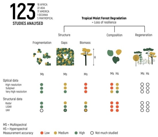
The research expressions (Table 1) encoded in Scopus in March 2019 matched with 919 articles (Figure 2). Sixteen relevant articles found by reading articles suggested by reviewers or published after the research, were added to the pool. In total, 10 duplicates were removed and abstract and title screening lead to the exclusion of 708 articles. Finally, 217 articles were fully read and 123 of them were selected to be part of the synthesis.
Two thirds of the studies selected in the final pool were localized in South or Central America. Degradation of other tropical forest basins is poorly studied (Figure 3). Most of the studies are carried out on a local or landscape scale on areas ranging from plots of a few hectares [53], to forest management unit (from 500 to 2000 hectares) [54,55], or areas delimited by remote sensing data acquisition footprint (e.g., Landsat tiles [56]). The few pantropical studies mainly focused on forest fragmentation [57,58,59], on degradation causes such as fires and logging [60] and on aboveground carbon density change [61]. There are still studies covering important surfaces. In the Congo basin, the area of forest loss due to disturbance drivers was estimated [27]. About 84% of forest degraded area is caused by small-scale and nonmechanized forest clearing for agriculture, followed by selective logging that accounts for 10%. In Amazonia, a regional biomass map was made by linking a canopy height model from remote sensing with an individual-based forest model [62]. Forest structure (basal area.ha−1, stem diameter, canopy height, number of trees.ha−1) variation caused by tree-level to regional-scale disturbances can be therefore quantified. It thus provides a basis for large-scale analyses on the heterogeneous structure of tropical forests and their carbon cycle. In Southeast Asia, a fragmentation map was made of the whole region. Plantations of rubber and palm oil were taken into account, which is important in this region which contains most of such plantations in the world [63].
The number of articles published about degradation remains stable until 2013, when a peak of 15 publications is noted (Figure 4). More than 50% of the studies were carried out after 2013 with an average increase of 10.4 studies compared to 3.8 studies in the year before 2013. The first studies, before 2004, took place in South America, more particularly in Brazil, and cover secondary forests [64], gold mining activities [65], fragmentation [66] and timber exploitation [67]. The number of articles on the Amazonian basin then increased steadily, with 3.9 studies per year, and remained the first studied zone compared to the other regions (Figure 4). The first study in the Congo basin was published in 2004 and concerned selective logging in the Central African Republic [68]. The average number of articles published per year remains very low for Central Africa, with a slight increase from 2013 onwards, from 0.4 (2004–2012) to 1.9 (2013–2019) studies per year. In Southeast Asia, the first study came later, in 2007, and concerns secondary forests [69]. The number of articles then increased continuously with an average of 1.7 (2007–2019) studies per year.
3.2. Indicators of Composition, Structure and Regeneration Measured with Remote Sensing
Among indicators of composition, structure and regeneration, structural indicators are the most used in studies monitoring tropical moist forest degradation (Table 2), particularly canopy gaps and landscape fragmentation. Fragmentation is the breaking of large, contiguous, forested areas into smaller pieces of forest and is influenced by large-scale phenomena e.g., roads extension, agriculture or mining developments [70]. Fragmentation appears to a large extent and so, is easily measurable with high-resolution (10–50 m) satellite data [63,71,72].
On the other hand, the detection and precise measurement of canopy gaps, which can appear at a smaller extent, requires LiDAR [73,74] data or very high-resolution optical images. In French Guiana, canopy gaps larger than 100 m² were detected using SPOT 5 images (10 m–resolution) [75]. In Ecuador, images coming from the same satellite were used to detect degraded forests with a canopy cover between 30% and 86% (general accuracy of 97.2%) [76]. In Costa Rica, canopy openings were detected (R² = 0.82 in relation to field data) on 26 plots of 0.25 hectares using a digital photogrammetric canopy height model (CHM), from UAV acquisition. In this study, portions of forests less than two meters in height were defined as a canopy opening [53].
High-resolution radar (SAR) data (10–50 m), although it offers good results [77], does not allow the detection of small disturbances [78]. High-resolution optical data underestimate canopy gaps [75]. More recently, Hethcoat et al. [79] developed a Random Forest machine-learning algorithm based on 30m Landsat images to detect pixels affected by timber harvesting in Brazil. This method allowed the detection of low-intensity selective logging (<15 m³.ha−1; 1–2 trees ha−1). Underestimation of canopy gaps can be limited by working at the sub-pixel level through spectral mixture analysis that provides different classes of fraction contained in a pixel [80].
A multitemporal approach also offers good results. In Brazil, Landsat 8 (30m-resolution) and Sentinel-2 (10m-resolution) imagery were used to detect canopy change caused by selective logging. They used a temporal approach by comparing images before and after disturbance. Both data show similar accuracy in selective logging detection with areas mapped as logged with Landsat imagery were considerably larger in comparison with Sentinel-2-based results [81]. In Cambodia and Laos, a comparison between two Landsat scenes was also performed to detect forest canopy disturbance and is able to highlight events as small as 0.005 ha [82]. In the Amazon Ecoregion, times series and sub-pixel analysis were performed on Landsat data to map deforestation, degradation and natural disturbance [83]. Finally, in Vietnam, the forest ecological vulnerability was assessed at the landscape scale [84]. Ecological vulnerability (V) depends on exposure to external stresses (E), sensitivity to perturbation (S) and capacity to recover or adapt (AC; V = S + E – AC) [85]. Imageries over 45 years (Landsat and Sentinel-2) were used to calculate indicators of S, E and AC based on evergreen forest, agricultural land proportion and fragmentation dynamics.
Above-ground biomass and carbon stock, integrating other structure parameters such as tree or stem diameter [86], are mainly used as indicators of forest degradation (Table 2). To model biomass, regressions between field measurements (e.g., above-ground biomass, volume, basal area, number of stems), at inventory plot or tree scale, and metrics from remote sensing data (aerial LiDAR [87], optical [88], radar [89]) are performed. In Borneo, above-ground biomass was calculated (Root mean square error (RMSE) = 20.3 tonnes.ha−1) by relating stem diameter to crown area. The crown was delineated by segmenting IKONOS images (1 to 4 m-resolution), with a segmentation accuracy of 39% for degraded forests [90]. Good results were also obtained by mixing different types of data, giving both spectral and structural information (optical and aerial LiDAR [91], optical and radar satellite with data saturation beyond 300 Mg.ha−1 [92]). In Myanmar, above-ground biomass variation, caused by selective logging, was measured using a photogrammetric digital surface model (DSM), from UAV acquisition, on two nine-hectare plots [93].
Measuring canopy height (CHM: Canopy Height Model, Table 2) with remote sensing requires normalizing the canopy top elevation (DSM) by subtracting the ground elevation (digital terrain model, DTM). This information (DTM and DSM) can be obtained using radar data according to the wavelength used: short wavelengths (e.g., X-band, λ ~ 3 cm) do not penetrate the vegetation and reflect the top of canopy, long wavelengths (e.g., L-band, λ ~ 23 cm and P-band, λ ~ 65 cm) pass through the vegetation and give information about the ground topography [77,94,95]. P-band could revolutionize forest structure knowledge around the world. This is the reason why the Biomass satellite (ESA mission, launch planned in 2022), that will be the first P-band SAR and the first radar tomographic space mission, will create a lot of opportunities. In some studies, SRTM (Shuttle Radar Topography Mission) of 30 to 90 m resolution, is used [77,94].
DSM and DTM can be calculated with very high accuracy by filtering upper and lower LiDAR returns [91,96]. When there are regular canopy gaps, the same discrimination can be achieved from photogrammetric point clouds, but with less accuracy. In Indonesia, a RMSE equal to 5 m to heights from LiDAR data was calculated on 48 and 82 hectares plots [97]. Another solution is to produce a DTM by interpolating GPS altimeter points taken in the field, which gives similar results to a DTM from LiDAR data [53]. The latter solution depends on the structure and nature of the forest cover, which will strongly influence the quality of reception of the GPS signal on the ground.
The compositional criterion is not commonly measured in articles studying the degradation of tropical moist forests that are structurally complex and rich in species, and so difficult to identify (Table 2). In Borneo, Landsat imagery cannot effectively detect subtle intra-guild trait variation (e.g., trait variation within climax guild) because of the low spatial/spectral resolution. However, Landsat imagery has been proven to be able to detect inter-guild trait differences (i.e., trait differences between pioneer and climax guilds). A composition gradient is then linked to a degradation gradient [98].
3.3. Remote Sensing Metrics and Indices Used to Detect Tropical Moist Forest Degradation
Metrics and indices can be calculated in order to highlight some aspects (e.g., soil, vegetation, height, granularity, etc.) of remote sensing data. In this study, textural metrics were first noted. In remote sensing, texture refers to the spatial variation of image greyscale levels. Visual and qualitative characteristics of an image, e.g., roughness, granularity or contrast, can be expressed with quantitative statistics measurement called textural metrics. Mobile windows, which are squares moving on the imagery, allow comparisons between pixels and its surroundings [104,105]. Two kinds of metrics are usually used: (1) the first-order ones that are statistical properties calculated within a certain window (e.g., the mean, the standard deviation, etc.) and therefore do not consider pixel neighbor relationships; (2) the second-order metrics that consider the spatial relations between groups of two neighboring pixels within the window. These last metrics are the most frequent in papers noted in this study. It requires calculating Gray-Level Co-occurrence Matrices (GLCM) which are “matrices containing the probabilities of co-occurrence of pixel values for pairs of pixels in a given direction and distance” [106]. The following second-order textural metrics were noted in this study [105,106,107,108]:
-
The variance which measures global variation in the image. Large values denote high levels of spectral heterogeneity (salt and pepper effect);
-
The contrast which is a quadratic measure of the local variation in the image. High values indicate large differences between neighboring pixels;
-
The dissimilarity which is a linear measure of the local variation in the image. Low values indicate homogenous texture;
-
The homogeneity which measures the uniformity of tones in the image. High values indicate homogenous texture;
-
The entropy which measures the disorder in the image. High values indicate disorder;
-
The angular second moment which measures the order in the image. High values indicate order;
-
The correlation which measures the linear dependency between neighboring pixels.
Spectral indices combine spectral reflectance from two or more wavelengths which indicates the relative abundance of features of interest. Vegetation index are the most common in studies measuring moist tropical forest degradation:
-
The “Enhanced Vegetation Index” (EVI) from MODIS satellite data is sensitive to canopy variations in high biomass regions where the “Normalized Difference Vegetation Index” (NDVI) saturates. When degradation is strong and closer to deforestation (e.g., fragmentation), the NDVI better highlights disturbances [111,112];
-
The “Global Environment Monitoring Index” (GEMI) was developed to assess vegetation by minimizing atmospheric effects and is sensitive to soil background [109,113]. Matricardi et al. [109] showed that a modified GEMI could be a reliable estimator of fractional canopy coverage, as well as the “Modified Soil Adjusted Vegetation Index aerosol resistant” (MSAVIaf) that minimizes soil background influences [114];
Some spectral indices directly focus on the disturbance (Table 3) such as the “Normalized Burn Ratio” (NBR) which highlights burned areas [119]. A difference between two NBR (ΔNBR) can also be used to assess forest disturbance that appears between two dates [81,82]. The “Forest Disturbance Index” (FDI) assumes that the soil of a disturbed forest will be more exposed than a conventional forest, resulting in more brightness and less wetness and greenness [120].
Sub-pixel spectral indices are also widely used to highlight disturbances in forest area. Through spectral mixture analysis, class fraction in a pixel can be extracted. Pure pixels, called endmembers, are used as spectral reference for each class. Their selection must be done carefully with the help of the “Pixel Purity Index” (PPI) for example [109]. For forest area, common classes are soil (SOIL), non-photosynthetic vegetation (NPV), green (GV), shadow and burned area (SHADE). Pixel fractions are then used to calculate sub-pixel indices (Table 3). The canopy gap fraction, measured on field, depends on the pixel green fraction calculated with the CLAS (Carnegie Landsat Analysis System) algorithm [121]. The “Normalized Difference Fraction Index” (NDFI) summarizes non-photosynthetic vegetation, green and soil fraction and is well adapted to selective logging and forest fires [122]. The forest degradation index (DEGRADI) underlines the spectral contrast between soil and green fraction in a pixel [123].
Polarimetric indices calculated from radar data [89,94,125] are also used. Indices commonly used are summarized and described in [89]: the parallel polarization ratio (Rpp) and the cross-polarization ratio (Rcp ) [126], the radar vegetation index (RVI) [127], the polarization fraction (PF) [128] and the pedestal height (PH) [129]. Some polarimetric indices are directly related to forest degradation and their compositional, structural and regeneration criteria (Table 4) such as the radar forest degradation index (RFDI) [89,130], the vegetation scattering index (VSI), the biomass index (BMI) and the canopy structure index (CSI) [131].
LiDAR and photogrammetric point clouds can be used to calculate metrics reflecting the 3D structure of the forest. Beyond statistical coefficients [87], other metrics can be calculated such as the “Relative Density Model” (RDM) [54] which detects whether the undergrowth, belonging to a user-defined range of heights, has been impacted (Figure 5). It is calculated by dividing the number of points between the upper and lower limit by the sum of these points with the number of points below the lower limit [54,87]. The “Topographic Position Index” (TPI) is an indicator of the topography, reflecting the position within the landscape (e.g., valley bottom or crest) [97]. The TPI is calculated with a moving window (150 × 150 m [97]) in which elevation of the central pixel (x) is compared to itself and the surrounding pixel elevation (X, n = 9).
4. Discussion
4.1. Temporal Evolution, Geographical Distribution and Spatial Extent of Forest Degradation Studies Using Remote Sensing Tools
The number of papers measuring tropical rainforest degradation by remote sensing is low, with only 123 papers meeting the inclusion criteria. In contrast to its counterpart, deforestation, which is now well documented and spatialized [15,132], degradation is less known because it is difficult to detect and poorly defined [9,133,134]. There is in fact no scientific consensus on the concept of forest degradation, leading to a large number of definitions and multiple ways of measuring it, particularly by remote sensing, as demonstrated in this literature review. Studying degradation from the point of view of forest dynamics and resilience opens up many opportunities and more challenges. This would make it possible, in particular, to generalize and isolate this definition from any preconceived ideas put forward by humans [36,37].
Tropical moist forest degradation is mainly studied and monitored in South America. The degradation of forests in Central Africa and Southeast Asia is hardly studied, which does not mean that the phenomenon is not present. This trend is not specific to degradation, but is also found in other fields of study, for example in hydrology [135] or in agroforestry [136]. However, degradation is more significant in the forests of Central Africa and Southeast Asia, where 65% and 63%, respectively, are considered as forests regenerated as a result of human activity [18]. In particular, the Congo Basin is experiencing pressure on the forests mainly due to its use by local populations for agriculture. With one exception in Gabon, where selective logging causes more damage than in other countries [27]. The other two tropical basins are experiencing more industrial forest exploitation, leading to deforestation, with palm plantations in Southeast Asia and cattle grazing facilities in South America [137,138]. Although an increase in the number of studies has been noted for Central Africa, from 2013 onwards, with an average of 1.9 papers per year instead of 0.4 before, knowledge about the degradation of the Congo Basin remains too low, as do other environmental and social areas [138].
4.2. Indicators of Composition, Structure and Regeneration Measured with Remote Sensing
In order to measure forest degradation in terms of its resilience, indicators of composition and structure make it possible to assess the state of the forest at time t. Regeneration indicators provide information about the capacity of the forest to recover by itself [37]. This study showed which indicators are usually measured in tropical rainforests, using remote sensing tools. Looking at forest composition, it is not widely studied with only one study in Borneo able to detect trait differences between pioneer and climax guilds using Landsat data [98]. In the literature [139], the results in detecting forest composition or its specific diversity vary according to the spatial and spectral resolution of data used [98,140]. The results can be bad to medium or good if multispectral [140] or hyperspectral [141,142] images, respectively, are used. Recently, in South America, studies using very high-resolution images acquired by UAVs show the potential of this tool to study the composition of tropical moist forests (RGB images [143], hyperspectral data [144]).
The main indicators measured by remote sensing in forest degradation studies are related to forest structure. Fragmentation and canopy gaps represent two different levels in the process of degradation. Canopy gaps are isolated disturbances that occur punctually in time, in the case of selective logging for example [145]. The presence of canopy gaps does not necessarily mean that the forest is degraded according to their size, number and frequency [73,146]. This process, called “gap dynamics” [147], occurs naturally in the forest dynamic cycle, during windfalls for example. Fragmentation, on the other hand, is the result of a longer process which persists over time [58,148], which is associated with deforestation and leads to other disturbance such as forest fires [149]. Canopy gaps can therefore be considered as punctual disturbances occurring before the tipping point, which if intensified or repeated over time, can lead to forest fragmentation. When the forest is fragmented, it has gone beyond the tipping point, has reached "degraded" status, and depending on the degree of fragmentation, is approaching deforestation. Biomass is another indicator of structure measured by remote sensing. Although it cannot be accurately measured to a large extent at present, it is an integrative parameter of the forest since it depends on height, tree diameter and wood density [86]. It can also be spatialized from other structural indicators, such as canopy gaps and canopy height [62]. Besides being a good degradation indicator, quantifying vegetation biomass enables the quantification of the amount of carbon stored by vegetation. In the context of global warming, this information can be used to calculate the carbon sequestration potential of forests under future climate and land use scenarios. Nowadays carbon in forests cannot be spatialized at a large scale. However, GEDI (launched in 2018 with data that should be released to the public in late fall 2019) satellite is collecting LiDAR data, while BIOMASS (launch in 2022) will collect radar data in P-band. Both will open new opportunities in forest monitoring.
In tropical moist forests, regeneration is poorly measured using remote sensing techniques. The age of the forest and the area covered by secondary forests, while constituting a first step in the characterization of regeneration, are not sufficient on their own. Indeed, being able to link the age as well as the successional stage of a forest with its structure, as recently done in Brazil [89], is essential, as well as characterizing the composition of regenerating trees [150]. Looking at other forests, LiDAR shows good results, for example, in undergrowth vegetation cover prediction [151]. UAV-imageries seem to be a potential niche for quickly, accurately, and reliably providing highly detailed spatial, spectral, and structural information on forest regeneration [152]. In addition to characterizing regeneration itself and when time series data are available, the main trajectory of a forest can be defined by looking at its state before and after disturbance as well as years following disturbance [81,84,93].
4.3. Remote Sensing Metrics and Indices Used to Detect Tropical Moist Forest Degradation
This study leads to the same conclusions as previous reviews on the subject [49,50]. Airborne LiDAR data add value to the quantification of degradation but are not available over large territories, to a large extent and at a high temporal frequency. Moreover, it is a costly tool for local actors. Optical and radar satellite data are more affordable and regularly available. High-resolution optical data can detect canopy gaps up to a certain size [79,80], especially when working at sub-pixel scale (Table 3) or with multitemporal data. They can help to measure biomass [88] and species composition [98]. However, image resolution limits the accuracy of the results. Very high-resolution optical data provide better results and opportunities for forest monitoring. They allow the detection of small disturbances (SPOT, WorldView-2, GeoEye-1) [75,153], the boundaries of tree crown on which the biomass depends (SPOT, WorldView-2) [90,154,155], the identification of tree species (WorldView-3) [156,157] or the measurement of biomass in combination with airborne LiDAR measurements (Planet Dove) [158,159]. These data are, however, not free of charge and are still dependent on the very numerous clouds in tropical regions, preventing regular monitoring via satellite data. Texture indices which process several pixels at a time allow to contextualize the information [104,105] and are complementary to widely used spectral indices. Using radar data and polarimetric indices can provide information about forest structure. Good results are obtained in monitoring degradation by mixing radar and optical data [92], although radar data are saturated in tropical moist forests with high biomass.
Data acquired by UAVs offer perspectives by providing both information about the structure of the forest (DSM) and about its spectral signature (at least very high-resolution RGB data) at rather low costs. Studies carried out in tropical forests show that this technology can be used to estimate biomass (Sumatra [97], Ecuador [160]), to detect changes in structure (Myanmar [93]), to monitor forest regeneration (Brazil [53], Costa Rica [161]), to characterize composition (Panama [143], Brazil [144]), to detect invasive plants (Hawaii [162]) or liana infestation (Malaysia [163]) and to locate emerging trees (Sumatra [164]). Other studies should be carried out in tropical moist forests to confirm this potential but also to test the contribution of UAVs to the measurement of forest attributes, currently requiring the installation of inventory plots, such as Lorey’s height, root mean square diameter, basal area, volume and number of stems per hectare (China [165], Canada [166]). Moreover, “UAS-mounted sensors offer an extraordinary opportunity to bridge the existing gap between field observations and traditional air- and space-borne remote sensing, by providing high spatial detail over relatively large areas in an entirely new capacity for enhanced temporal retrieval”[167]. Beyond its use by scientists, the UAV which is more accessible financially [167] and easy to use, can be taken in hand by local communities and stakeholders (CBFM: Community-Based Forest Monitoring [51], CREMA: Community REsource Management Area [138]), making it possible to acquire data at a high temporal frequency and to participate in forest monitoring [52]. This tool is a good way to help local populations manage their forests and to promote the implementation of UN sustainable development goals, which must be implemented at different scales in order to be reached [29].
When the forest cover is dense, it is not always possible to produce a DTM by filtering the photogrammetric point cloud [97,168]. Sufficiently large, numerous and well-distributed canopy gaps over the study area, in which soil is visible, are required. These conditions are difficult to reach in tropical moist forests where the forest cover is dense. Other methods must then be considered in order to obtain altimetric data to normalize the DSMs produced, such as the interpolation of GPS altimeter points taken in the field [53], the use of topographic indices (TPI) [97] or the use of a DTM derived from other data such as the SRTM [77,94], which are less accurate. Ideally, methods that do not require DTMs should be established [161]. Finally, UAV technology is evolving quickly and shows good potential even though the spatial extent that can be covered remains limited compared to satellite data [169]. An interesting lead would be to evaluate how UAV data can be linked to satellite data to cover a larger spatial extent, as has been performed in temperate [170] and boreal [171] forests.
5. Conclusions
There are today multiple ways to define forest degradation leading to many interpretations. Using the concept of resilience to study forest degradation creates many opportunities and isolates the definition from any preconceived ideas. Especially, degradation criteria (i.e., composition, structure, regeneration) should be monitored. Using remote sensing seems to be a must in rainforests, which are difficult to access and cover large areas. However, tropical moist forest degradation is today poorly studied, especially in the Congo Basin which is experiencing significant pressure on its forests from the agricultural activity of local populations.
Structure is the most measured criteria by remote sensing. Fragmentation, which is an advanced stage of degradation, is now well monitored using high-resolution satellite data. Accurate measurement of canopy gaps and biomass requires LiDAR or very high-resolution data. As tropical moist forests are complex and contain lots of diversity, composition is poorly measured with the quality of measurement linked to data resolution and the use of hyperspectral data. Finally, regeneration is not yet well characterized using remote sensing tools.
This study shows the large panel of indices (spectral, textural, polarimetric) used to measure tropical moist forest degradation. A lot of data are now available and mixing different types (LiDAR or radar and optical data) leads to good results. Very high-resolution satellites provide precious information for forest monitoring. Performant satellites giving accurate information on tropical moist forest structure are missing but the gap should soon be filled by the awaited GEDI and BIOMASS data. LiDAR and UAVs form a good bridge between field and satellite data. While the performance of the LiDAR is no longer to be demonstrated, of particular interest should be the UAV which has great potential and would be easily used by local communities and stakeholders.
Author Contributions
Conceptualization, C.D., P.L., A.M. and A.F.; methodology, C.D., P.L. and A.F.; validation, C.D., P.L., A.M. and A.F.; formal analysis, C.D.; investigation, C.D.; resources, C.D.; data curation, C.D.; writing—original draft preparation, C.D., P.L., A.M. and A.F.; writing—review and editing, C.D.; visualization, C.D.; supervision, C.D., P.L. and A.F.; project administration, C.D., P.L., and A.F.; All authors have read and agreed to the published version of the manuscript.
Funding
This research received no external funding.
Acknowledgments
We thank Clément Dupuis for the proofreading in English and Alix Gancille for the drawing of the diagrams. We also thank the reviewers, especially reviewer 1, who suggested interesting articles to add to our analysis.
Conflicts of Interest
The authors declare no conflict of interest.
References
- IPCC. Global Warming of 1.5 °C—An IPCC Special Report on the Impacts of Global Warming of 1.5 °C above Pre-Industrial Levels and Related Global Greenhouse Gas Emission Pathways, in the Context of Strengthening the Global Response to the Threat of Climate Chang; IPCC: Incheon, Korea, 2018. [Google Scholar]
- IPBES. Report of the Plenary of the Intergovernmental Science-Policy Platform on Biodiversity and Ecosystem Services on the Work of Its Seventh Session; IPBES: Paris, France, 2019. [Google Scholar]
- Ceballos, G.; Ehrlich, P.R.; Dirzo, R. Biological Annihilation via the Ongoing Sixth Mass Extinction Signaled by Vertebrate Population Losses and Declines. PNAS 2017, 114, 6089–6096. [Google Scholar] [CrossRef] [PubMed] [Green Version]
- Lewis, S.L.; Edwards, D.P.; Galbraith, D. Increasing Human Dominance of Tropical Forests. Science 2015, 349, 827–832. [Google Scholar] [CrossRef] [PubMed]
- Costanza, R.; D’Arge, R.; de Groot, R.; Farber, S.; Grasso, M.; Hannon, B.; Limburg, K.; Naeem, S.; O’Neill, R.V.; Paruelo, J.; et al. The Value of the World’s Ecosystem Services and Natural Capital. Nature 1997, 387, 253–260. [Google Scholar] [CrossRef]
- FAO. Assessing Forest Degradation—Towards the Development of Globally Applicable Guidlines; FAO: Rome, Italy, 2011. [Google Scholar] [CrossRef]
- Pan, Y.; Birdsey, R.; Fang, J.; Houghton, R.; Kauppi, P.E.; Kurz, W.A.; Phillips, O.L.; Shvidenko, A.; Lewis, S.L.; Canadell, J.G.; et al. A Large and Persistent Carbon Sink in the World’s Forests. Science 2011, 333, 988–994. [Google Scholar] [CrossRef] [Green Version]
- Mitchard, E.T.A. The Tropical Forest Carbon Cycle and Climate Change. Nature 2018, 559, 527–534. [Google Scholar] [CrossRef]
- Pearson, T.R.H.; Brown, S.; Murray, L.; Sidman, G. Greenhouse Gas Emissions from Tropical Forest Degradation: An Underestimated Source. Carbon Balance Manag. 2017, 12, 1–11. [Google Scholar] [CrossRef] [PubMed] [Green Version]
- Abernethy, K.; Maisels, F.; White, L.J.T. Environmental Issues in Central Africa. Annu. Rev. Environ. Resour. 2016, 41, 1–33. [Google Scholar] [CrossRef] [Green Version]
- Achard, F.; Beuchle, R.; Mayaux, P.; Stibig, H.J.; Bodart, C.; Brink, A.; Carboni, S.; Desclée, B.; Donnay, F.; Eva, H.D.; et al. Determination of Tropical Deforestation Rates and Related Carbon Losses from 1990 to 2010. Glob. Chang. Biol. 2014, 20, 2540–2554. [Google Scholar] [CrossRef]
- Tyukavina, A.; Baccini, A.; Hansen, M.C.; Potapov, P.V.; Stehman, S.V.; Houghton, R.A.; Krylov, A.M.; Turubanova, S.; Goetz, S.J. Aboveground Carbon Loss in Natural and Managed Tropical Forests from 2000 to 2012. Environ. Res. Lett. 2015, 10. [Google Scholar] [CrossRef]
- Hubau, W.; Lewis, S.; Phillips, O.; Affum-Baffoe, K.; Beeckman, H.; Cuní-Sanchez, A.; Daniels, A.; Ewango, C.; Fauset, S.; Mukinzi, J.; et al. Asynchronous Carbon Sink Saturation in African and Amazonian Tropical Forests. Nature 2020, 579, 80–87. [Google Scholar] [CrossRef] [Green Version]
- Keenan, R.J.; Reams, G.A.; Achard, F.; de Freitas, J.V.; Grainger, A.; Lindquist, E. Dynamics of Global Forest Area: Results from the FAO Global Forest Resources Assessment 2015. For. Ecol. Manag. 2015, 352, 9–20. [Google Scholar] [CrossRef]
- Song, X.; Hansen, M.C.; Stephen, V.; Peter, V.; Tyukavina, A.; Vermote, E.F.; Townshend, J.R. Global Land Change from 1982 to 2016. Nature 2018, 560, 639–643. [Google Scholar] [CrossRef] [PubMed]
- Morales-Hidalgo, D.; Oswalt, S.N.; Somanathan, E. Status and Trends in Global Primary Forest, Protected Areas, and Areas Designated for Conservation of Biodiversity from the Global Forest Resources Assessment 2015. For. Ecol. Manag. 2015, 352, 68–77. [Google Scholar] [CrossRef] [Green Version]
- Potapov, P.; Hansen, M.C.; Laestadius, L.; Turubanova, S.; Yaroshenko, A.; Thies, C.; Smith, W.; Zhuravleva, I.; Komarova, A.; Minnemeyer, S.; et al. The Last Frontiers of Wilderness: Tracking Loss of Intact Forest Landscapes from 2000 to 2013. Sci. Adv. 2017, 3, 1–14. [Google Scholar] [CrossRef] [Green Version]
- FAO. The State of Forests in the Amazon Basin, Congo Basin and Southeast Asia; FAO: Brazzaville, Republic of Congo, 2011. [Google Scholar]
- Tapia-Armijos, M.F.; Homeier, J.; Espinosa, C.I.; Leuschner, C.; De La Cruz, M. Deforestation and Forest Fragmentation in South Ecuador since the 1970s—Losing a Hotspot of Biodiversity. PLoS ONE 2015, 10, 1–18. [Google Scholar] [CrossRef] [Green Version]
- Barlow, J.; Lennox, G.D.; Ferreira, J.; Berenguer, E.; Lees, A.C.; Nally, R.M.; Thomson, J.R.; Ferraz, S.F.D.B.; Louzada, J.; Oliveira, V.H.F.; et al. Anthropogenic Disturbance in Tropical Forests Can Double Biodiversity Loss from Deforestation. Nature 2016, 535, 144–147. [Google Scholar] [CrossRef] [Green Version]
- Karamage, F.; Shao, H.; Chen, X.; Ndayisaba, F.; Nahayo, L.; Kayiranga, A.; Omifolaji, J.K.; Liu, T.; Zhang, C. Deforestation Effects on Soil Erosion in the Lake Kivu Basin, D.R. Congo-Rwanda. Forests 2016, 7, 281. [Google Scholar] [CrossRef] [Green Version]
- Celentano, D.; Rousseau, G.X.; Engel, V.L.; Zelarayán, M.; Oliveira, E.C.; Araujo, A.C.M.; de Moura, E.G. Degradation of Riparian Forest Affects Soil Properties and Ecosystem Services Provision in Eastern Amazon of Brazil. L. Degrad. Dev. 2016, 28, 482–493. [Google Scholar] [CrossRef]
- Priess, J.A.; Mimler, M.; Klein, A.-M.; Schwarze, S.; Tscharntke, T.; Steffan-Dewenter, I. Linking Deforestation Scenarios to Pollination Services and Economic Returns in Coffee Agroforestery Systems. Ecol. Appl. 2007, 17, 407–417. [Google Scholar] [CrossRef] [Green Version]
- Ehara, M.; Hyakumura, K.; Nomura, H.; Matsuura, T.; Sokh, H.; Leng, C. Identifying Characteristics of Households Affected by Deforestation in Their Fuelwood and Non-Timber Forest Product Collections: Case Study in Kampong Thom Province, Cambodia. Land Use Policy 2016, 52, 92–102. [Google Scholar] [CrossRef]
- Burkett-Cadena, N.D.; Vittor, A.Y. Deforestation and Vector-Borne Disease: Forest Conversion Favors Important Mosquito Vectors of Human Pathogens. Basic Appl. Ecol. 2018, 26, 101–110. [Google Scholar] [CrossRef]
- Van der Werf, G.R.; Morton, D.C.; DeFries, R.S.; Olivier, J.G.J.; Kasibhatla, P.S.; Jackson, R.B.; Collatz, G.J.; Randerson, J.T. CO2 Emissions from Forest Loss. Nat. Geosci. 2009, 2, 737–738. [Google Scholar] [CrossRef]
- Tyukavina, A.; Hansen, M.C.; Potapov, P.; Parker, D.; Okpa, C.; Stehman, S.V.; Kommareddy, I.; Turubanova, S. Congo Basin Forest Loss Dominated by Increasing Smallholder Clearing. Sci. Adv. 2018, 4, 1–12. [Google Scholar] [CrossRef] [PubMed] [Green Version]
- Kissinger, G.; Herold, M.; De Sy, V. Drivers of Deforestation and Forest Degradation: A Synthesis Report for REDD+ Policymakers; The Government of the UK and Norway: Vancouver, Canada, 2012. [Google Scholar] [CrossRef]
- The United Nations. Sustainable Development Goals. Available online: https://www.un.org/sustainabledevelopment/ (accessed on 30 January 2020).
- FAO; UNDP; UNEP. UN-REDD Programme Strategic Framework 2016–2020 (UNREDD/PB14/2015/III/3); UN-REDD Programme fourteenth policy board meeting; Washington, DC, USA, 2015; Available online: https://www.google.com.hk/url?sa=t&rct=j&q=&esrc=s&source=web&cd=1&ved=2ahUKEwi7zviqp7zoAhUNUd4KHe1fCTkQFjAAegQIAhAB&url=http%3A%2F%2Fwww.redd-monitor.org%2Fwp-content%2Fuploads%2F2016%2F11%2FUNREDD_PB14_2015_Strategic-Framework-2016-20-7May2015-130662-1.pdf&usg=AOvVaw01YNiuUx0MuY4OH1UYDtqB (accessed on 12 January 2020).
- Ochieng, R.M.; Visseren-Hamakers, I.J.; Arts, B.; Brockhaus, M.; Herold, M. Institutional Effectiveness of REDD+ MRV: Countries Progress in Implementing Technical Guidelines and Good Governance Requirements. Environ. Sci. Policy 2016, 61, 42–52. [Google Scholar] [CrossRef] [Green Version]
- Simula, M. Vers Une Définition de La Dégradation Des Forêts: Analyse Comparative Des Définitions Existantes; FAO: Rome, Italy, 2009. [Google Scholar]
- Arana Pardo, J.I.; Birdsey, R.; Boehm, M.; Daka, J.; Kobayashi, S.; Lund, H.G.; Michalak, R.; Takahashi, M. IPCC Report on Definitions and Methodological Options to Inventory Emissions from Direct Human-Induced Degradation of Forests and Devegetation of Other Vegetation Types; Institute for Global Environmental Strategies: Hayama, Kanagawa, Japan, 2003; ISBN 4-88788-004-9. [Google Scholar]
- FAO. Global Forest Resources Assessment 2020: Terms and Definition; FAO: Rome, Italy, 2018. [Google Scholar]
- ITTO. ITTO Guidelines for the Restoration, Management and Rehabilitation of Degraded and Secondary Tropical Forests; ITTO Policy Development Series No 13; ITTO: Yokohama, Kanagawa, Japan, 2002. [Google Scholar]
- Ghazoul, J.; Burivalova, Z.; Garcia-Ulloa, J.; King, L.A. Conceptualizing Forest Degradation. Trends Ecol. Evol. 2015, 30, 622–632. [Google Scholar] [CrossRef]
- Vásquez-Grandón, A.; Donoso, P.J.; Gerding, V. Forest Degradation: When Is a Forest Degraded? Forests 2018, 9, 726. [Google Scholar] [CrossRef] [Green Version]
- Ghazoul, J.; Chazdon, R. Degradation and Recovery in Changing Forest Landscapes: A Multiscale Conceptual Framework. Annu. Rev. Environ. Resour. 2017, 42, 161–188. [Google Scholar] [CrossRef] [Green Version]
- Gourlet-Fleury, S.; Mortier, F.; Fayolle, A.; Baya, F.; Ouédraogo, D.; Bénédet, F.; Picard, N. Tropical Forest Recovery from Logging: A 24 Year Silvicultural Experiment from Central Africa. Philos. Trans. R. Soc. B 2013, 368, 1–10. [Google Scholar] [CrossRef] [Green Version]
- Doucet, J.; Daïnou, K.; Ligot, G.; Ouédraogo, D.; Bourland, N.; Ward, S.E.; Tekam, P.; Lagoute, P.; Fayolle, A.; Bourland, N.; et al. Enrichment of Central African Logged Forests with High-Value Tree Species: Testing a New Approach to Regenerating Degraded Forests. Int. J. Biodivers. Sci. Ecosyst. Serv. Manag. 2016, 12, 83–95. [Google Scholar] [CrossRef] [Green Version]
- Poorter, L.; Bongers, F.; Aide, T.M.; Almeyda Zambrano, A.M.; Balvanera, P.; Becknell, J.M.; Boukili, V.; Brancalion, P.H.S.; Broadbent, E.N.; Chazdon, R.L.; et al. Biomass Resilience of Neotropical Secondary Forests. Nature 2016, 530, 211–214. [Google Scholar] [CrossRef]
- Thompson, I.D.; Guariguata, M.R.; Okabe, K.; Bahamondez, C.; Nasi, R.; Heymell, V.; Sabogal, C. An Operational Framework for Defining and Monitoring Forest Degradation. Ecol. Soc. 2013, 18. [Google Scholar] [CrossRef]
- Standish, R.J.; Hobbs, R.J.; Mayfield, M.M.; Bestelmeyer, B.T.; Suding, K.N.; Battaglia, L.L.; Eviner, V.; Hawkes, C.V.; Temperton, V.M.; Cramer, V.A.; et al. Resilience in Ecology: Abstraction, Distraction, or Where the Action Is? Biol. Conserv. 2014, 177, 43–51. [Google Scholar] [CrossRef] [Green Version]
- IPCC. 2019 Refinement To the 2006 IPCC Guidelines for National Greenhouse Gas Inventories; IPCC: Geneva, Switzerland, 2019. [Google Scholar] [CrossRef]
- GOFC-GOLD. A Sourcebook of Methods and Procedures for Monitoring and Reporting Anthropogenic Greenhouse Gas Emissions and Removals Associated with Deforestation, Gains and Losses of Carbon Stocks in Forests Remaining Forests, and Forestation; GOFC-GOLD Land Cover Project Office: Wageningen, The Netherlands, 2016. [Google Scholar]
- GFOI. Integration of Remote-Sensing and Ground-Based Observations for Estimation of Emissions and Removals of Greenhouse Gases in Forests: Methods and Guidance from the Global Forest Observations Initiative, 2nd ed.; GFOI: Rome, Italy, 2016. [Google Scholar]
- Sanchez-Azofeifa, A.; Antonio Guzmán, J.; Campos, C.A.; Castro, S.; Garcia-Millan, V.; Nightingale, J.; Rankine, C. Twenty-First Century Remote Sensing Technologies Are Revolutionizing the Study of Tropical Forests. Biotropica 2017, 49, 604–619. [Google Scholar] [CrossRef]
- Finer, M.; Novoa, S.; Weisse, J.; Petersen, R.; Souto, T.; Stearns, F.; Martinez, R.G. Combating Deforestation: From Satellite to Intervention. Science 2018, 360, 1303–1305. [Google Scholar] [CrossRef] [PubMed]
- Mitchell, A.L.; Rosenqvist, A.; Mora, B. Current Remote Sensing Approaches to Monitoring Forest Degradation in Support of Countries Measurement, Reporting and Verification (MRV) Systems for REDD+. Carbon Balance Manag. 2017, 12. [Google Scholar] [CrossRef] [PubMed] [Green Version]
- Joseph, S.; Murthy, M.S.R.; Thomas, A.P. The Progress on Remote Sensing Technology in Identifying Tropical Forest Degradation: A Synthesis of the Present Knowledge and Future Perspectives. Environ. Earth Sci. 2011, 64, 731–741. [Google Scholar] [CrossRef]
- Fry, B.P. Community Forest Monitoring in REDD +: The ‘M’ in MRV? Environ. Sci. Policy 2011, 14, 181–187. [Google Scholar] [CrossRef]
- Paneque-gálvez, J.; Mccall, M.K.; Napoletano, B.M.; Wich, S.A.; Koh, L.P. Small Drones for Community-Based Forest Monitoring: An Assessment of Their Feasibility and Potential in Tropical Areas. Forests 2014, 5, 1481–1507. [Google Scholar] [CrossRef] [Green Version]
- Zahawi, R.A.; Dandois, J.P.; Holl, K.D.; Nadwodny, D.; Reid, J.L.; Ellis, E.C. Using Lightweight Unmanned Aerial Vehicles to Monitor Tropical Forest Recovery. Biol. Conserv. 2015, 186, 287–295. [Google Scholar] [CrossRef] [Green Version]
- de Carvalho, A.L.; D’Oliveria, M.V.N.; Putz, F.E.; de Oliveira, L.C. Natural Regeneration of Trees in Selectively Logged Forest in Western Amazonia. For. Ecol. Manag. 2017, 392, 36–44. [Google Scholar] [CrossRef] [Green Version]
- Sufo Kankeu, R.; Sonwa, D.J.; Eba’a Atyi, R.; Moankang Nkal, N.M. Quantifying Post Logging Biomass Loss Using Satellite Images and Ground Measurements in Southeast Cameroon. J. For. Res. 2016, 27, 1415–1426. [Google Scholar] [CrossRef]
- Shimabukuro, Y.E.; Beuchle, R.; Grecchi, R.C. Assessment of Forest Degradation in Brazilian Amazon Due to Selective Logging and Fires Using Time Series of Fraction Images Derived from Landsat ETM + Images. Remote Sens. Lett. 2014, 5, 773–782. [Google Scholar] [CrossRef]
- Brinck, K.; Fischer, R.; Lehmann, S.; De Paula, M.D.; Putz, S.; Sexton, J.O.; Song, D.; Huth, A. High Resolution Analysis of Tropical Forest Fragmentation and Its Impact on the Global Carbon Cycle. Nat. Commun. 2017, 8. [Google Scholar] [CrossRef] [PubMed] [Green Version]
- Taubert, F.; Fischer, R.; Groeneveld, J.; Lehmann, S.; Müller, M.S.; Rödig, E.; Wiegand, T.; Huth, A. Global Patterns of Tropical Forest Fragmentation. Nature 2018, 554, 519–522. [Google Scholar] [CrossRef] [PubMed]
- Wade, T.G.; Riitters, K.H.; Wickham, J.D.; Jones, K.B. Distribution and Causes of Global Forest Fragmentation. Conserv. Ecol. 2003, 7, 1–5. Available online: http://www.consecol.org/vol7/iss2/art7/ (accessed on 5 January 2020). [CrossRef]
- Tyukavina, A.; Hansen, M.C.; Potapov, P.V.; Krylov, A.M.; Goetz, S.J. Pan-Tropical Hinterland Forests: Mapping Minimally Disturbed Forests. Glob. Ecol. Biogeogr. 2016, 25, 151–163. [Google Scholar] [CrossRef]
- Baccini, A.; Walker, W.; Carvalho, L.; Farina, M.; Houghton, R.A. Tropical Forests Are a Net Carbon Source Based on Aboveground Measurements of Gain and Loss. Science 2017, 358, 230–234. [Google Scholar] [CrossRef] [Green Version]
- Rodig, E.; Cuntz, M.; Heinke, J.; Rammig, A.; Huth, A. Spatial Heterogeneity of Biomass and Forest Structure of the Amazon Rain Forest: Linking Remote Sensing, Forest Modelling and Field Inventory. Glob. Ecol. Biogeogr. 2017, 26, 1292–1302. [Google Scholar] [CrossRef]
- Dong, J.; Xiao, X.; Sheldon, S.; Biradar, C.; Zhang, G.; Duong, N.D.; Hazarika, M.; Wikantika, K.; Takeuhci, W.; Moore, B. A 50-m Forest Cover Map in Southeast Asia from ALOS / PALSAR and Its Application on Forest Fragmentation Assessment. PLoS ONE 2014, 9. [Google Scholar] [CrossRef] [Green Version]
- Lucas, R.M.; Honzák, M.; Curran, P.J.; Foody, G.M.; Nguele, D.T. Characterizing Tropical Forest Regeneration in Cameroon Using NOAA AVHRR Data. Int. J. Remote Sens. 2000, 21, 2831–2854. [Google Scholar] [CrossRef]
- Almeida-filho, R.; Shimabukuro, Y.E. Detecting Areas Disturbed by Gold Mining Activities through JERS-1 SAR Images, Roraima State, Brazilian Amazon. Int. J. Remote Sens. 2000, 21, 3357–3362. [Google Scholar] [CrossRef]
- Cochrane, M.A.; Laurance, W.F. Fire as a Large-Scale Edge Effect in Amazonian Forests. J. Trop. Ecol. 2002, 18, 311–325. [Google Scholar] [CrossRef] [Green Version]
- Asner, G.P.; Keller, M.; Pereira, R.; Zweede, J.C. Remote Sensing of Selective Logging in Amazonia Assessing Limitations Based on Detailed Field Observations, Landsat ETM +, and Textural Analysis. Remote Sens. Environ. 2002, 80, 483–496. [Google Scholar] [CrossRef]
- De Wasseige, C.; Defourny, P. Remote Sensing of Selective Logging Impact for Tropical Forest. Manag. For. Ecol. Manag. 2004, 188, 161–173. [Google Scholar] [CrossRef]
- Tottrup, C.; Rasmussen, M.S.; Eklundh, L.; Jönsson, P. Mapping Fractional Forest Cover across the Highlands of Mainland Southeast Asia Using MODIS Data and Regression Tree Modelling. Int. J. Remote Sens. 2007, 28, 23–46. [Google Scholar] [CrossRef]
- Laurance, W.F.; Camargo, J.L.C.; Fearnside, P.M.; Lovejoy, T.E.; Williamson, G.B.; Mesquita, R.C.G.; Meyer, C.F.J.; Bobrowiec, P.E.D.; Laurance, S.G.W. An Amazonian Rainforest and Its Fragments as a Laboratory of Global Change. Biol. Rev. 2018, 93, 223–247. [Google Scholar] [CrossRef]
- Da Ponte, E.; Roch, M.; Leinenkugel, P.; Dech, S.; Kuenzer, C. Paraguay’s Atlantic Forest Cover Loss e Satellite-Based Change Detection and Fragmentation Analysis between 2003 and 2013. Appl. Geogr. 2017, 79, 37–49. [Google Scholar] [CrossRef]
- Broadbent, E.N.; Asner, G.P.; Keller, M.; Knapp, D.E.; Oliveira, P.J.C.; Silva, J.N. Forest Fragmentation and Edge Effects from Deforestation and Selective Logging in the Brazilian Amazon. Biol. Conserv. 2008, 141, 1745–1757. [Google Scholar] [CrossRef]
- Asner, G.P.; Kellner, J.R.; Kennedy-Bowdoin, T.; Knapp, D.E.; Anderson, C.; Martin, R.E. Forest Canopy Gap Distributions in the Southern Peruvian Amazon. PLoS ONE 2013, 8, 1–10. [Google Scholar] [CrossRef] [Green Version]
- Boyd, D.S.; Hill, R.A.; Hopkinson, C.; Baker, T.R. Landscape-Scale Forest Disturbance Regimes in Southern Peruvian Amazonia. Ecol. Soc. Am. 2017, 23, 1588–1602. [Google Scholar] [CrossRef]
- Pithon, S.; Jubelin, G.; Guitet, S.; Gond, V. A Statistical Method for Detecting Logging-Related Canopy Gaps Using High-Resolution Optical Remote Sensing. Int. J. Remote Sens. 2013, 34, 700–711. [Google Scholar] [CrossRef]
- Delgado-aguilar, M.J.; Hinojosa, L.; Schmitt, C.B. Combining Remote Sensing Techniques and Participatory Mapping to Understand the Relations between Forest Degradation and Ecosystems Services in a Tropical Rainforest. Appl. Geogr. 2019, 104, 65–74. [Google Scholar] [CrossRef]
- Deutscher, J.; Perko, R.; Gutjahr, K.; Hirschmugl, M.; Schardt, M. Mapping Tropical Rainforest Canopy Disturbances in 3D by COSMO-SkyMed Spotlight InSAR-Stereo Data to Detect Areas of Forest Degradation. Remote Sens. 2013, 5, 648–663. [Google Scholar] [CrossRef] [Green Version]
- Joshi, N.; Mitchard, E.T.A.; Woo, N.; Torres, J.; Moll-Rocek, J.; Ehammer, A.; Collins, M.; Jepsen, M.R.; Fensholt, R. Mapping Dynamics of Deforestation and Forest Degradation in Tropical Forests Using Radar Satellite Data. Environ. Res. Lett. 2015, 10. [Google Scholar] [CrossRef] [Green Version]
- Hethcoat, M.G.; Edwards, D.P.; Carreiras, J.M.B.; Bryant, R.G.; França, F.M.; Quegan, S. A Machine Learning Approach to Map Tropical Selective Logging. Remote Sens. Environ. 2019, 221, 569–582. [Google Scholar] [CrossRef]
- Pinagé, E.R.; Matricardi, E.A.T.; Leal, F.A.; Pedlowski, M.A. Estimates of Selective Logging Impacts in Tropical Forest Canopy Cover Using RapidEye Imagery and Field Data. iForest 2016, 9, 461–468. [Google Scholar] [CrossRef] [Green Version]
- Lima, T.A.; Beuchle, R.; Langner, A.; Grecchi, R.C.; Griess, V.C.; Achard, F. Comparing Sentinel-2 MSI and Landsat 8 OLI Imagery for Monitoring Selective Logging in the Brazilian Amazon. Remote Sens. 2019, 11, 961. [Google Scholar] [CrossRef] [Green Version]
- Langner, A.; Miettinen, J.; Kukkonen, M.; Vancutsem, C.; Simonetti, D.; Vieilledent, G.; Verhegghen, A.; Gallego, J.; Stibig, H.J. Towards Operational Monitoring of Forest Canopy Disturbance in Evergreen Rain Forests: A Test Case in Continental Southeast Asia. Remote Sens. 2018, 10, 544. [Google Scholar] [CrossRef] [Green Version]
- Bullock, E.L.; Woodcock, C.E.; Souza, C.; Olofsson, P. Satellite-Based Estimates Reveal Widespread Forest Degradation in the Amazon. Glob. Chang. Biol. 2020, 1–14. [Google Scholar] [CrossRef]
- Bourgoin, C.; Oszwald, J.; Bourgoin, J.; Gond, V.; Blanc, L.; Dessard, H.; Van Phan, T.; Sist, P.; Läderach, P.; Reymondin, L. Assessing the Ecological Vulnerability of Forest Landscape to Agricultural Frontier Expansion in the Central Highlands of Vietnam. Int. J. Appl. Earth Obs. Geoinf. 2020, 84. [Google Scholar] [CrossRef]
- Fritzsche, K.; Schneiderbauer, S.; Bubeck, P.; Kienberger, S.; Buth, M.; Zebisch, M.; Kahlenborn, W. The Vulnerability Sourcebook: Concept and Guidelines for Standardised Vulnerability Assessments; Deutsche Gesellschaft für Internationale Zusammenarbeit: Bonn and Eschborn, Germany, 2014. [Google Scholar]
- Chave, J.; Réjou-Méchain, M.; Búrquez, A.; Chidumayo, E.; Colgan, M.S.; Delitti, W.B.C.; Duque, A.; Eid, T.; Fearnside, P.M.; Goodman, R.C.; et al. Improved Allometric Models to Estimate the Aboveground Biomass of Tropical Trees. Glob. Chang. Biol. 2014, 20, 3177–3190. [Google Scholar] [CrossRef] [PubMed]
- D’Oliveira, M.V.N.; Reutebuch, S.E.; Mcgaughey, R.J.; Andersen, H. Estimating Forest Biomass and Identifying Low-Intensity Logging Areas Using Airborne Scanning Lidar in Antimary State Forest, Acre State, Western Brazilian Amazon. Remote Sens. Environ. 2012, 124, 479–491. [Google Scholar] [CrossRef]
- Pfeifer, M.; Kor, L.; Nilus, R.; Turner, E.; Cusack, J.; Lysenko, I.; Khoo, M.; Chey, V.K.; Chung, A.C.; Ewers, R.M. Mapping the Structure of Borneo’s Tropical Forests across a Degradation Gradient. Remote Sens. Environ. 2016, 176, 84–97. [Google Scholar] [CrossRef] [Green Version]
- Cassol, H.L.G.; Carreiras, D.B.; Moraes, E.C.; Eduardo, L.; De Arag, C.; Val, C.; Silva, D.J.; Quegan, S.; Shimabukuro, Y.E. Retrieving Secondary Forest Aboveground Biomass from Polarimetric ALOS-2 PALSAR-2 Data in the Brazilian Amazon. Remote Sens. 2019, 11, 59. [Google Scholar] [CrossRef] [Green Version]
- Phua, M.H.; Ling, Z.Y.; Coomes, D.A.; Wong, W.; Korom, A.; Tsuyuki, S.; Ioki, K.; Hirata, Y.; Saito, H.; Takao, G. Seeing Trees from Space: Above-Ground Biomass Estimates of Intact and Degraded Montane Rainforests from High-Resolution Optical Imagery. IForest 2017, 10, 625–634. [Google Scholar] [CrossRef] [Green Version]
- Rappaport, D.I.; Morton, D.C.; Longo, M.; Keller, M.; Dubayah, R.; Dos-Santos, M.N. Quantifying Long-Term Changes in Carbon Stocks and Forest Structure from Amazon Forest Degradation Quantifying Long-Term Changes in Carbon Stocks and Forest Structure from Amazon Forest Degradation. Environ. Res. Lett. 2018, 13. [Google Scholar] [CrossRef]
- Bourgoin, C.; Blanc, L.; Bailly, J.-S.; Cornu, G.; Berenguer, E.; Oszwald, J.; Tritsch, I.; Laurent, F.F.; Hasan, A.; Sist, P.; et al. The Potential of Multisource Remote Sensing for Mapping the Biomass of a Degraded Amazonian Forest. Forests 2018, 9, 303. [Google Scholar] [CrossRef] [Green Version]
- Ota, T.; Ahmed, O.S.; Thu, S.; Cin, T.; Mizoue, N.; Yoshida, S. Estimating Selective Logging Impacts on Aboveground Biomass in Tropical Forests Using Digital Aerial Photography Obtained before and after a Logging Event from an Unmanned Aerial Vehicle. For. Ecol. Manage. 2019, 433, 162–169. [Google Scholar] [CrossRef]
- Carreiras, J.M.B.; Jones, J.; Lucas, R.M.; Shimabukuro, Y.E. Mapping Major Land Cover Types and Retrieving the Age of Secondary Forests in the Brazilian Amazon by Combining Single-Date Optical and Radar Remote Sensing Data. Remote Sens. Environ. 2017, 194, 16–32. [Google Scholar] [CrossRef] [Green Version]
- Deutscher, J.; Gutjahr, K.; Perko, R.; Raggam, H.; Hirschmugl, M.; Schardt, M. Humid Tropical Forest Monitoring with Multi-Temporal L-, C- and X-Band SAR Data. In Proceedings of the 2017 9th International Workshop on the Analysis of Multitemporal Remote Sensing Images (MultiTemp), Brugge, Belgium, 27–29 June 2017. [Google Scholar] [CrossRef]
- Kronseder, K.; Ballhorn, U.; Böhmc, V.; Siegert, F. Above Ground Biomass Estimation across Forest Types at Different Degradation Levels in Central Kalimantan Using Lidar Data. Int. J. Appl. Earth Obs. Geoinf. 2012, 18, 37–48. [Google Scholar] [CrossRef]
- Swinfield, T.; Lindsell, J.A.; Williams, J.V.; Harrison, R.D.; Gemita, E.; Schönlieb, C.B.; Coomes, D.A. Accurate Measurement of Tropical Forest Canopy Heights and Aboveground Carbon Using Structure From Motion. Remote Sens. 2019, 11, 928. [Google Scholar] [CrossRef] [Green Version]
- Fujiki, S.; Aoyagi, R.; Tanaka, A.; Imai, N.; Kusma, A.D.; Kurniawan, Y.; Lee, Y.F.; Sugau, J.B.; Pereira, J.T.; Samejima, H.; et al. Large-Scale Mapping of Tree-Community Composition as a Surrogate of Forest Degradation in Bornean Tropical Rain Forests. Land 2016, 5, 45. [Google Scholar] [CrossRef] [Green Version]
- Delgado-Aguilar, M.J.; Fassnacht, F.E.; Peralvo, M.; Gross, C.P.; Schmitt, C.B. Potential of TerraSAR-X and Sentinel 1 Imagery to Map Deforested Areas and Derive Degradation Status in Complex Rain Forests of Ecuador. Int. For. Rev. 2017, 19, 102–118. [Google Scholar] [CrossRef]
- Putz, S.; Groeneveld, J.; Henle, K.; Knogge, C.; Martensen, A.C.; Metz, M.; Metzger, J.P.; Ribeiro, M.C.; Dantas de Paula, M.; Huth, A. Long-Term Carbon Loss in Fragmented Neotropical Forests. Nat. Commun. 2014, 5, 1–8. [Google Scholar] [CrossRef] [Green Version]
- Asner, G.P.; Powell, G.V.N.; Mascaro, J.; Knapp, D.E.; Clark, J.K.; Jacobson, J.; Kennedy-Bowdoin, T.; Balaji, A.; Paez-Acosta, G.; Victoria, E.; et al. High-Resolution Forest Carbon Stocks and Emissions in the Amazon. PNAS 2010, 107, 16738–16742. [Google Scholar] [CrossRef] [Green Version]
- Becknell, J.M.; Keller, M.; Piotto, D.; Longo, M.; Dos-Santos, M.N.; Scaranello, M.A.; de Oliveira Cavalcante, R.B.; Porder, S. Landscape-Scale Lidar Analysis of Aboveground Biomass Distribution in Secondary Brazilian Atlantic Forest. Biotropica 2018, 50, 520–530. [Google Scholar] [CrossRef]
- Fokeng, R.M.; Gadinga, W.; Meli, V.; Nyuyki, B. Multi-Temporal Forest Cover Change Detection in the Metchie-Ngoum Protection Forest Reserve, West Region of Cameroon. Egypt. J. Remote Sens. Sp. Sci. 2018. [Google Scholar] [CrossRef]
- Galvão, L.S.; dos Santos, J.R.; da Silva, R.D.; da Silva, C.V.; Moura, Y.M.; Breunig, F.M. Following a Site-Specific Secondary Succession in the Amazon Using the Landsat CDR Product and Field Inventory Data. Int. J. Remote Sens. 2015, 36, 574–596. [Google Scholar] [CrossRef]
- da Silva, R.D.; Galvão, L.S.; Santos, J.R.; Silva, C.V.D.J.; de Moura, Y.M. Spectral/Textural Attributes from ALI / EO-1 for Mapping Primary and Secondary Tropical Forests and Studying the Relationships with Biophysical Parameters. GIScience Remote Sens. 2014, 51, 677–694. [Google Scholar] [CrossRef]
- Lebrija-trejos, E.E.; Marco, A.; Gallardo-cruz, J.A.; Meave, J.A.; Gonza, E.J.; Herna, L.; Gallardo-cruz, R.; Pe, E.A.; Martorell, C. Predicting Tropical Dry Forest Successional Attributes from Space: Is the Key Hidden in Image Texture ? PLoS ONE 2012, 7, 38–45. [Google Scholar] [CrossRef] [Green Version]
- Haralick, R.M.; Shanmugam, K.; Dinstein, I. Textural Features for Image Classification. IEEE Trans. Syst. Man. Cybern. 1973, 3, 610–621. [Google Scholar] [CrossRef] [Green Version]
- Dedieu, J.-P.; Bornicchia, F.; Kerkache, R.; Pella, H. Apport Des Informations de Texture En Télédétection Pour l’étude de l’occupation Des Sols/The Contribution to Land-Use Studies of Textural Analysis Using Remote Sensing Data. Rev. Géographie Alp. 1997, 85, 9–26. [Google Scholar] [CrossRef]
- Matricardi, E.A.T.; Skole, D.L.; Pedlowski, M.A.; Chomentowski, W.; Fernandes, L.C. Assessment of Tropical Forest Degradation by Selective Logging and Fire Using Landsat Imagery. Remote Sens. Environ. 2010, 114, 1117–1129. [Google Scholar] [CrossRef]
- Karnieli, A.; Kaufman, Y.J.; Remer, L.; Wald, A. AFRI—Aerosol Free Vegetation Index. Remote Sens. Environ. 2001, 77, 10–21. [Google Scholar] [CrossRef]
- Huete, A.; Didan, K.; Miura, T.; Rodriguez, E.P.; Gao, X.; Ferreira, L.G. Overview of the Radiometric and Biophysical Performance of the MODIS Vegetation Indices. Remote Sens. Lett. 2002, 83, 195–213. [Google Scholar] [CrossRef]
- Ferreira, N.C.; Ferreira, L.G.; Huete, A.R. Assessing the Response of the MODIS Vegetation Indices to Landscape Disturbance in the Forested Areas of the Legal Brazilian Amazon. Int. J. Remote Sens. 2010, 31, 745–759. [Google Scholar] [CrossRef]
- Pinty, B.; Verstraete, M.M. GEMI: A Non-Linear Index to Monitor Global Vegetation from Satellites. Vegetatio 1992, 101, 15–20. [Google Scholar] [CrossRef]
- Qi, J.; Chehbouni, A.; Huete, A.R.; Kerr, Y.H.; Sorooshian, S. A Modified Soil Adjusted Vegetation Index. Remote Sens. Environ. 1994, 48, 119–126. [Google Scholar] [CrossRef]
- Bourbier, L.; Cornu, G.; Pennec, A.; Brognoli, C.; Gond, V. Large-Scale Estimation of Forest Canopy Opening Using Remote Sensing in Central Africa. Bois Forêts des Trop. 2013, 315, 3–9. [Google Scholar] [CrossRef] [Green Version]
- Motohka, T.; Nasahara, K.N.; Oguma, H.; Tsuchida, S. Applicability of Green-Red Vegetation Index for Remote Sensing of Vegetation Phenology. Remote Sens. 2010, 2, 2369–2387. [Google Scholar] [CrossRef] [Green Version]
- Gao, B.-C. NDWI—A Normalized Difference Water Index for Remote Sensing of Vegetation Liquid Water from Space. Remote Sens. Env. 1996, 58, 257–266. [Google Scholar] [CrossRef]
- Carreiras, M.B.; Jones, J.; Lucas, R.M.; Gabriel, C. Land Use and Land Cover Change Dynamics across the Brazilian Amazon: Insights from Extensive Time-Series Analysis of Remote Sensing Data. PLoS ONE 2014, 9, 1–24. [Google Scholar] [CrossRef] [PubMed]
- Sofan, P.; Vetrita, Y.; Yulianto, F.; Khomarudin, M.R. Multi-Temporal Remote Sensing Data and Spectral Indices Analysis for Detection Tropical Rainforest Degradation: Case Study in Kapuas Hulu and Sintang Districts, West Kalimantan, Indonesia. Nat. Hazards 2016, 80, 1279–1301. [Google Scholar] [CrossRef]
- Ghulam, A.; Ghulam, O.; Maimaitijiang, M.; Freeman, K.; Porton, I.; Maimaitiyiming, M. Remote Sensing Based Spatial Statistics to Document Tropical Rainforest Transition Pathways. Remote Sens. 2015, 7, 6257–6279. [Google Scholar] [CrossRef] [Green Version]
- Asner, G.P.; Broadbent, E.N.; Oliveira, P.J.C.; Keller, M.; Knapp, D.E.; Silva, J.N.M. Condition and Fate of Logged Forests in the Brazilian Amazon. PNAS 2006, 103, 12947–12950. [Google Scholar] [CrossRef] [PubMed] [Green Version]
- Souza, C.M.; Roberts, D.A.; Cochrane, M.A. Combining Spectral and Spatial Information to Map Canopy Damage from Selective Logging and Forest Fires. Remote Sens. Environ. 2005, 98, 329–343. [Google Scholar] [CrossRef]
- Pinheiro, T.F.; Escada, M.I.S.; Valeriano, D.M.; Hostert, P.; Gollnow, F.; Müller, H. Forest Degradation Associated with Logging Frontier Expansion in the Amazon: The BR-163 Region in Southwestern Pará, Brazil. Earth Interact. 2016, 20, 1–26. [Google Scholar] [CrossRef]
- Ji, L.; Zhang, L.; Wylie, B.K.; Rover, J. On the Terminology of the Spectral Vegetation Index (NIR−SWIR)/(NIR+SWIR). J. Remote Sens. 2011, 32, 6901–6909. [Google Scholar] [CrossRef]
- Mermoz, S.; Le Toan, T. Forest Disturbances and Regrowth Assessment Using ALOS PALSAR Data from 2007 to 2010 in Vietnam, Cambodia and Lao PDR. Remote Sens. 2016, 8, 217. [Google Scholar] [CrossRef] [Green Version]
- Pope, K.O.; Rey-Benayas, J.M.; Paris, J.F. Radar Remote Sensing of Forest and Wetland Ecosystems in the Central American Tropics. Remote Sens. Environ. 1994, 48, 205–219. [Google Scholar] [CrossRef]
- Freeman, A.; Durden, S. A Three-Component Scattering Model for Polarimetric SAR Data. IEEE Trans. Geosci. Remote Sens. 1998, 36, 936–973. [Google Scholar] [CrossRef] [Green Version]
- Durden, S.; van Zyl, J.; Zebker, H. The Unpolarized Component in Polarimetric Radar Observations of Forested Areas. IEEE Trans. Geosci. Remote Sens. 1990, 28, 268–271. [Google Scholar] [CrossRef]
- Allain, S.; Ferro-Famil, L.; Pottier, E. New Eigenvalue-Based Parameters for Natural Media Characterization. In Proceedings of the European Radar Conference 2005 (EURAD 2005), Paris, France, 3–4 October 2005. [Google Scholar]
- Henderson, F.M.; Lewis, A.J. Principles and Applications of Imaging Radar, Manual of Remote Sensing, 3rd ed.; Wiley: New York, NY, USA, 1999; Volume 80. [Google Scholar] [CrossRef]
- Ainsworth, T.L.; Lee, J.S.; Schuler, D.L. Multi-Frequency Polarimetric SAR Data Analysis of Ocean Surface Features. In Proceedings of the International Geoscience and Remote Sensing Symposium IGARS, Honolulu, HI, USA, 24–28 July 2000; pp. 1113–1115. [Google Scholar]
- Hansen, M.C.C.; Potapov, P.V.; Moore, R.; Hancher, M.; Turubanova, S.A.; Tyukavina, A.; Thau, D.; Stehman, S.V.V.; Goetz, S.J.J.; Loveland, T.R.R.; et al. High-Resolution Global Maps Of. Science 2013, 342, 850–854. [Google Scholar] [CrossRef] [PubMed] [Green Version]
- Lund, H.G. What Is a Degraded Forest? White Paper Prepared for FAO: Gainesville, VA, USA, 2009. [Google Scholar]
- Sasaki, N.; Putz, F.E. Critical Need for New Definitions of “Forest” and “Forest Degradation” in Global Climate Change Agreements. Conserv. Lett. 2009, 2, 226–232. [Google Scholar] [CrossRef]
- Lele, S. Watershed Services of Tropical Forests: From Hydrology to Economic Valuation to Integrated Analysis. Curr. Opin. Environ. Sustain. 2009, 1, 148–155. [Google Scholar] [CrossRef]
- De Beenhouwer, M.; Aerts, R.; Honnay, O. A Global Meta-Analysis of the Biodiversity and Ecosystem Service Benefits of Coffee and Cacao Agroforestry. Agric. Ecosyst. Environ. 2013, 175, 1–7. [Google Scholar] [CrossRef]
- Seymour, F.; Harris, N.L. Reducing Tropical Deforestation. Science 2019, 365, 756–757. [Google Scholar] [CrossRef] [Green Version]
- Malhi, Y.; Adu-Bredu, S.; Asare, R.A.; Lewis, S.L.; Mayaux, P. African Rainforests: Past, Present and Future. Philos. Trans. R. Soc. B Biol. Sci. 2013, 368, 1–10. [Google Scholar] [CrossRef] [Green Version]
- Ganivet, E.; Bloomberg, M. Towards Rapid Assessments of Tree Species Diversity and Structure in Fragmented Tropical Forests: A Review of Perspectives Offered by Remotely-Sensed and Field-Based Data. For. Ecol. Manag. 2019, 432, 40–53. [Google Scholar] [CrossRef]
- Wallis, C.I.B.; Brehm, G.; Donoso, D.A.; Fiedler, K.; Homeier, J.; Paulsch, D.; Süßenbach, D.; Tiede, Y.; Brandl, R.; Farwig, N.; et al. Remote Sensing Improves Prediction of Tropical Montane Species Diversity but Performance Differs among Taxa. Ecol. Indic. 2017, 83, 538–549. [Google Scholar] [CrossRef]
- Schäfer, E.; Heiskanen, J.; Heikinheimo, V.; Pellikka, P. Mapping Tree Species Diversity of a Tropical Montane Forest by Unsupervised Clustering of Airborne Imaging Spectroscopy Data. Ecol. Indic. 2016, 64, 49–58. [Google Scholar] [CrossRef]
- Féret, J.; Asner, G.P. Mapping Tropical Forest Canopy Diversity Using High-Fidelity Imaging Spectroscopy. Ecol. Soc. Am. 2014, 24, 1289–1296. [Google Scholar] [CrossRef] [PubMed]
- Park, J.Y.; Muller-Landau, H.C.; Lichstein, J.W.; Rifai, S.W.; Dandois, J.P.; Bohlman, S.A. Quantifying Leaf Phenology of Individual Trees and Species in a Tropical Forest Using Unmanned Aerial Vehicle (UAV) Images. Remote Sens. 2019, 11, 1534. [Google Scholar] [CrossRef] [Green Version]
- Sothe, C.; Dalponte, M.; de Almeida, C.M.; Schimalski, M.B.; Lima, C.L.; Liesenberg, V.; Miyoshi, G.T.; Tommaselli, A.M.G. Tree Species Classification in a Highly Diverse Subtropical Forest Integrating UAV-Based Photogrammetric Point Cloud and Hyperspectral Data. Remote Sens. 2019, 11, 1338. [Google Scholar] [CrossRef] [Green Version]
- Hirschmugl, M.; Steinegger, M.; Gallaun, H.; Schardt, M. Mapping Forest Degradation Due to Selective Logging by Means of Time Series Analysis: Case Studies in Central Africa. Remote Sens. 2014, 6, 756–775. [Google Scholar] [CrossRef] [Green Version]
- Matricardi, E.A.T.; Skole, D.L.; Pedlowski, M.A. Assessment of Forest Disturbances by Selective Logging and Forest Fires in the Brazilian Amazon Using Landsat Data. Int. J. Remote Sens. 2013, 34, 1057–1086. [Google Scholar] [CrossRef]
- Muscolo, A.; Bagnato, S.; Sidari, M.; Mercurio, R. A Review of the Roles of Forest Canopy Gaps. J. For. Res. 2014, 25, 725–736. [Google Scholar] [CrossRef]
- Newman, M.E.; Mclaren, K.P.; Wilson, B.S. Assessing Deforestation and Fragmentation in a Tropical Moist Forest over 68 Years; the Impact of Roads and Legal Protection in the Cockpit Country, Jamaica. For. Ecol. Manag. 2014, 315, 138–152. [Google Scholar] [CrossRef]
- Junior, C.H.L.S.; Arag, L.E.O.C.; Fonseca, M.G.; Almeida, C.T.; Vedovato, L.B.; Id, L.O.A. Deforestation-Induced Fragmentation Increases Forest Fire Occurrence in Central Brazilian Amazonia. Forests 2018, 9, 305. [Google Scholar] [CrossRef] [Green Version]
- Helmer, E.H.; Ruzycki, T.S.; Wilson, B.T.; Sherrill, K.R.; Lefsky, M.A.; Marcano-Vega, H.; Brandeis, T.J.; Erickson, H.E.; Ruefenacht, B. Tropical Deforestation and Recolonization by Exotic and Native Trees: Spatial Patterns of Tropical Forest Biomass, Functional Groups, and Species Counts and Links to Stand Age, Geoclimate, and Sustainability Goals. Remote Sens. 2018, 10, 1724. [Google Scholar] [CrossRef] [Green Version]
- Wing, B.M.; Ritchie, M.W.; Boston, K.; Cohen, W.B.; Gitelman, A.; Olsen, M.J. Prediction of Understory Vegetation Cover with Airborne Lidar in an Interior Ponderosa Pine Forest. Remote Sens. Environ. 2012, 124, 730–741. [Google Scholar] [CrossRef]
- Goodbody, T.R.H.; Coops, N.C.; Hermosilla, T.; Tompalski, P.; Crawford, P. Assessing the Status of Forest Regeneration Using Digital Aerial Photogrammetry and Unmanned Aerial Systems. Int. J. Remote Sens. 2018, 39, 5246–5264. [Google Scholar] [CrossRef]
- Dalagnol, R.; Phillips, O.L.; Gloor, E.; Galvão, L.S.; Wagner, F.H.; Locks, C.J.; Aragão, L.E.O.C. Quantifying Canopy Tree Loss and Gap Recovery in Tropical Forests under Low-Intensity Logging Using VHR Satellite Imagery and Airborne LiDAR. Remote Sens. 2019, 11, 817. [Google Scholar] [CrossRef] [Green Version]
- Loubota Panzou, G.J.; Fayolle, A.; Feldpausch, T.R.; Ligot, G.; Doucet, J.L.; Forni, E.; Zombo, I.; Mazengue, M.; Loumeto, J.J.; Gourlet-Fleury, S. What Controls Local-Scale Aboveground Biomass Variation in Central Africa? Testing Structural, Composition and Architectural Attributes. For. Ecol. Manag. 2018, 429, 570–578. [Google Scholar] [CrossRef]
- Wagner, F.H.; Ferreira, M.P.; Sanchez, A.; Hirye, M.C.M.; Zortea, M.; Gloor, E.; Phillips, O.L.; de Souza Filho, C.R.; Shimabukuro, Y.E.; Aragão, L.E.O.C. Individual Tree Crown Delineation in a Highly Diverse Tropical Forest Using Very High Resolution Satellite Images. ISPRS J. Photogramm. Remote Sens. 2018, 145, 362–377. [Google Scholar] [CrossRef]
- Cross, M.; Scambos, T.; Pacifici, F.; Vargas-Ramirez, O.; Moreno-Sanchez, R.; Marshall, W. Classification of Tropical Forest Tree Species Using Meter-Scale Image Data. Remote Sens. 2019, 11, 1411. [Google Scholar] [CrossRef] [Green Version]
- Ferreira, M.P.; Wagner, F.H.; Aragão, L.E.O.C.; Shimabukuro, Y.E.; de Souza Filho, C.R. Tree Species Classification in Tropical Forests Using Visible to Shortwave Infrared WorldView-3 Images and Texture Analysis. ISPRS J. Photogramm. Remote Sens. 2019, 149, 119–131. [Google Scholar] [CrossRef]
- Csillik, O.; Asner, G.P. Aboveground Carbon Emissions from Gold Mining in the Peruvian Amazon Aboveground Carbon Emissions from Gold Mining in the Peruvian Amazon. Environ. Res. Lett. 2020, 15, 1–11. [Google Scholar] [CrossRef]
- Csillik, O.; Kumar, P.; Mascaro, J.; O’Shea, T.; Asner, G.P. Monitoring Tropical Forest Carbon Stocks and Emissions Using Planet Satellite Data. Sci. Rep. 2019, 9, 1–12. [Google Scholar] [CrossRef] [Green Version]
- González-Jaramillo, V.; Fries, A.; Bendix, J. AGB Estimation in a Tropical Mountain Forest (TMF) by Means of RGB and Multispectral Images Using an Unmanned Aerial Vehicle (UAV). Remote Sens. 2019, 11, 1413. [Google Scholar] [CrossRef] [Green Version]
- Berveglieri, A.; Imai, N.N.; Tommaselli, A.M.G.; Casagrande, B.; Honkavaara, E. Successional Stages and Their Evolution in Tropical Forests Using Multi- Temporal Photogrammetric Surface Models and Superpixels. ISPRS J. Photogramm. Remote Sens. 2018, 146, 548–558. [Google Scholar] [CrossRef]
- Perroy, R.L.; Sullivan, T.; Stephenson, N. Assessing the Impacts of Canopy Openness and Flight Parameters on Detecting a Sub-Canopy Tropical Invasive Plant Using a Small Unmanned Aerial System. ISPRS J. Photogramm. Remote Sens. 2017, 125, 174–183. [Google Scholar] [CrossRef]
- Waite, C.E.; van der Heijden, G.M.F.; Field, R.; Boyd, D.S. A View from above: Unmanned Aerial Vehicles (UAVs) Provide a New Tool for Assessing Liana Infestation in Tropical Forest Canopies. J. Appl. Ecol. 2019, 56, 902–912. [Google Scholar] [CrossRef]
- Alexander, C.; Korstjens, A.H.; Hankinson, E.; Usher, G.; Harrison, N.; Nowak, M.G.; Abdullah, A.; Wich, S.A.; Hill, R.A. Locating Emergent Trees in a Tropical Rainforest Using Data from an Unmanned Aerial Vehicle (UAV). Int. J. Appl. Earth Obs. Geoinf. 2018, 72, 86–90. [Google Scholar] [CrossRef]
- Xu, Z.; Li, W.; Li, Y.; Shen, X.; Ruan, H. Estimation of Secondary Forest Parameters by Integrating Image and Point Cloud-Based Metrics Acquired from Unmanned Aerial Vehicle. J. Appl. Remote Sens. 2019, 14, 1–17. [Google Scholar] [CrossRef] [Green Version]
- Tompalski, P.; White, J.C.; Coops, N.C.; Wulder, M.A. Quantifying the Contribution of Spectral Metrics Derived from Digital Aerial Photogrammetry to Area-Based Models of Forest Inventory Attributes. Remote Sens. Environ. 2019, 234, 1–13. [Google Scholar] [CrossRef]
- Manfreda, S.; McCabe, M.F.; Miller, P.E.; Lucas, R.; Madrigal, V.P.; Mallinis, G.; Dor, E.B.; Helman, D.; Estes, L.; Ciraolo, G.; et al. On the Use of Unmanned Aerial Systems for Environmental Monitoring. Remote Sens. 2018, 10, 641. [Google Scholar] [CrossRef] [Green Version]
- Anders, N.; Valente, J.; Masselink, R.; Keesstra, S. Comparing Filtering Techniques for Removing Vegetation from UAV-Based Photogrammetric Point Clouds. Drones 2019, 3, 61. [Google Scholar] [CrossRef] [Green Version]
- Colomina, I.; Molina, P. Unmanned Aerial Systems for Photogrammetry and Remote Sensing: A Review. ISPRS J. Photogramm. Remote Sens. 2014, 92, 79–97. [Google Scholar] [CrossRef] [Green Version]
- Abdollahnejad, A.; Panagiotidis, D.; Surovỳ, P. Estimation and Extrapolation of Tree Parameters Using Spectral Correlation between UAV and Pléiades Data. Forests 2018, 9, 85. [Google Scholar] [CrossRef] [Green Version]
- Puliti, S.; Saarela, S.; Gobakken, T.; Ståhl, G.; Næsset, E. Combining UAV and Sentinel-2 Auxiliary Data for Forest Growing Stock Volume Estimation through Hierarchical Model-Based Inference. Remote Sens. Environ. 2018, 204, 485–497. [Google Scholar] [CrossRef]
Figure 1. Forest transition curve illustrating the degradation process through the frame of resilience. The indicator of composition, structure and regeneration used to evaluate the degradation reflect the resilience of forests [37]. The curve illustrates variation of an indicator and its recovery to a reference state after a disturbance (A). If the disturbance is more intense, the indicator will take more time to recover (B), as well as if disturbances appear more frequently (C). Intense and/or frequent disturbances can lead the forest to a tipping point from which the forest will head towards a degraded state. The indicator value is below an expected level and the forest is considered as degraded. The curve 1, 2 and 3 represent different levels of forest degradation (adapted from [37,42,43]).
Figure 1. Forest transition curve illustrating the degradation process through the frame of resilience. The indicator of composition, structure and regeneration used to evaluate the degradation reflect the resilience of forests [37]. The curve illustrates variation of an indicator and its recovery to a reference state after a disturbance (A). If the disturbance is more intense, the indicator will take more time to recover (B), as well as if disturbances appear more frequently (C). Intense and/or frequent disturbances can lead the forest to a tipping point from which the forest will head towards a degraded state. The indicator value is below an expected level and the forest is considered as degraded. The curve 1, 2 and 3 represent different levels of forest degradation (adapted from [37,42,43]).

Figure 2. Study flow diagram (PRISMA) showing the flow of information through the different phases of the systematic review.
Figure 2. Study flow diagram (PRISMA) showing the flow of information through the different phases of the systematic review.

Figure 3. Frequency of articles according to their geographical area and their spatial extent.

Figure 4. Relative cumulative frequency of articles according to time and to their geographical zone.
Figure 4. Relative cumulative frequency of articles according to time and to their geographical zone.

Figure 5. Illustration of relative density model (RDM) calculation method (Number of returns between the upper and lower RDM limits/Number of returns between the ground level and the upper RDM limits). (A) The RDM is equal to 0/(0 + 3) = 0, indicating that the undergrowth has been crushed or removed. (B) The RDM is equal to 7/(7 + 3) = 0.7, indicating intact undergrowth with little or no disturbance of vegetation in the 1–5 m range of heights. (C) The RDM is equal to 0/(0 + 0) = undefined, indicating the forest is very dense, with an intact canopy not disturbed.
Figure 5. Illustration of relative density model (RDM) calculation method (Number of returns between the upper and lower RDM limits/Number of returns between the ground level and the upper RDM limits). (A) The RDM is equal to 0/(0 + 3) = 0, indicating that the undergrowth has been crushed or removed. (B) The RDM is equal to 7/(7 + 3) = 0.7, indicating intact undergrowth with little or no disturbance of vegetation in the 1–5 m range of heights. (C) The RDM is equal to 0/(0 + 0) = undefined, indicating the forest is very dense, with an intact canopy not disturbed.


Table 1. Search expression encoded in Scopus database (March 2019) and applied to titles, abstracts and keywords.
Table 1. Search expression encoded in Scopus database (March 2019) and applied to titles, abstracts and keywords.
| Criteria | Search Expression | |
|---|---|---|
| What? | degraded OR degradation OR disturbed OR disturbance OR altered OR alteration OR “secondary forest*” OR regeneration OR succession OR “second-growth forest*” OR “second growth forest*” OR “regrowth forest*” OR fragmented OR fragmentation OR “canopy gap*” | |
| How? | AND | “remote sensing” OR lidar OR satellite OR sar OR radar OR image* OR uav OR “unmanned aerial vehicle” |
| Where? | AND | rainforest* OR jungle OR “tropical moist forest*” OR “equatorial forest*” OR “tropical humid forest*” OR “rain forest*” OR “central Africa” OR “congo basin” OR amazon* OR “southeast asia” |
| Limited to? Date range |
Articles 2000 to present |
|
Table 2. Indicators of composition, structure and regeneration with the number of articles using them and examples in the references column.
Table 2. Indicators of composition, structure and regeneration with the number of articles using them and examples in the references column.
| Indicators | Number of Articles | References |
|---|---|---|
| Structure | ||
| Canopy cover | 2 | [99] |
| Canopy gaps and cutting area | 12 | [79] |
| Landscape fragmentation (patches number, area and perimeter, fractal dimension) | 17 | [57,58,72,100] |
| Forest density | 1 | [63] |
| Connectivity | 1 | [63] |
| Above-ground biomass and carbon stock | 22 | [101] |
| Canopy height | 4 | [102] |
| Composition Pioneer and climax species groups |
1 | [98] |
| Regeneration | ||
| Secondary forest age | 8 | [94] |
| Area of secondary forests Succession stage |
3 10 |
[103] [89] |
Table 3. Spectral indices used in the detection of tropical moist forest degradation.
| Indices | Description | Reference |
|---|---|---|
| - at pixel scale | ||
| Normalized Burn Ratio (NBR) |
where SWIR wavelength is between 2.05 and 2.45 μm [124] |
[119,124] |
| Forest Disturbance Index (DI) | [120] | |
| - at sub-pixel scale | ||
| Canopy gap fraction | Depends on gap fraction and needing calibration with field data | [121] |
| Normalized Difference Fraction Index (NDFI) | Adapted to selective logging and forest fires: where: |
[122] |
| Forest Degradation Index (DEGRADI) | Highlights disturbed forests area: |
[123] |
Table 4. Polarimetric indices used in the detection of tropical moist forest degradation.
| Indices | Description | References |
|---|---|---|
| Radar Forest Degradation Index (RFDI) |
Highlights canopy cover variation: |
[89,130] |
| Biomass Index (BMI) |
Links leaf (crown) biomass to woody biomass: |
[89,131] |
| Canopy Structure Index (CSI) |
Relative importance of vertical versus horizontal structure of vegetation: |
[89,131] |
| Vegetation Scattering Index (VSI) | Canopy thickness and density indicator: |
[89,131] |
où:
: backscatter coefficient in decibel dB, polarization HH: horizontal electric wave for both emission and reception, polarization HV: horizontal electric wave for emission and electric wave for reception, polarization VV: vertical electric wave for both emission and reception.
© 2020 by the authors. Licensee MDPI, Basel, Switzerland. This article is an open access article distributed under the terms and conditions of the Creative Commons Attribution (CC BY) license (http://creativecommons.org/licenses/by/4.0/).
Share and Cite
MDPI and ACS Style
Dupuis, C.; Lejeune, P.; Michez, A.; Fayolle, A. How Can Remote Sensing Help Monitor Tropical Moist Forest Degradation?—A Systematic Review. Remote Sens. 2020, 12, 1087. https://doi.org/10.3390/rs12071087
AMA Style
Dupuis C, Lejeune P, Michez A, Fayolle A. How Can Remote Sensing Help Monitor Tropical Moist Forest Degradation?—A Systematic Review. Remote Sensing. 2020; 12(7):1087. https://doi.org/10.3390/rs12071087
Chicago/Turabian StyleDupuis, Chloé, Philippe Lejeune, Adrien Michez, and Adeline Fayolle. 2020. "How Can Remote Sensing Help Monitor Tropical Moist Forest Degradation?—A Systematic Review" Remote Sensing 12, no. 7: 1087. https://doi.org/10.3390/rs12071087
Note that from the first issue of 2016, this journal uses article numbers instead of page numbers. See further details here.