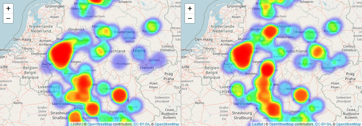
In this code example I use a geocoding function found on datascienceplus to geocode Google trends search intensity data, comparing search trend by city name for “Burger” and “Pizza” in Germany. I then visualize the results with heatmaps, generated with the Leaflet package in R.

Geocoding input data using Open Street Map API

In below coding example I implement the geocoding function from “datascienceplus” and apply it using two DataFrames with Google Trends data. The DataFrames contain tabular data retrieved from the Google Trends service, comprising search intensity scores by German city names for the search terms “Burger” and “Pizza”.

# implementing a geocoding function, using JSON-based OSM-API
#install.packages("jsonlite")
library(jsonlite)

# documentation: http://wiki.openstreetmap.org/wiki/Nominatim
# source: 
# datascienceplus.com/osm-nominatim-with-r-getting-locations-geo-coordinates-by-its-address/
osm_geocoder <- function(address = NULL)
{
  if(suppressWarnings(is.null(address)))
    return(data.frame())
  
  tryCatch(
    d <- jsonlite::fromJSON( 
      gsub('\\@addr\\@', gsub('\\s+', '\\%20', address), 
           'http://nominatim.openstreetmap.org/search/@addr@?format=json&addressdetails=0&limit=1')
    ), error = function(c) return(data.frame())
  )

  if(length(d) == 0) 
    return(data.frame())
  
  return(data.frame(lon = as.numeric(d$lon), lat = as.numeric(d$lat)))
}

# reading input data (tabular csv files with Google Trends data 
setwd("C:/Users/Linnart/Desktop/Supply Chain Analytics/08 R coding/01__spatial visualization/Spatial food trends analysis")

# input data comprises Google search intensity for burger and pizza in Germany
input_pizza_map <- read.csv(file="Pizza on map.csv",header=TRUE,sep=",",stringsAsFactors = FALSE)
input_burger_map <- read.csv(file="Burger on map.csv",header=TRUE,sep=",",stringsAsFactors = FALSE)
#input_burger_and_pizza_map <-read.csv(file="Pizza vs Burger on map.csv",header=TRUE,sep=",",stringsAsFactors = FALSE)
#input_burger_and_pizza_timeline <- read.csv(file="Pizza vs Burger.csv",header=TRUE,sep=",",stringsAsFactors = FALSE)

# geocoding input data, i.e. applying the geo-coding function
input_pizza_map<-data.frame(input_pizza_map$Town.City,"Lat"=rep(NA,nrow(input_pizza_map)),"Long"=rep(NA,nrow(input_pizza_map)),input_pizza_map$Pizza...2.12.17...2.12.18.)
input_burger_map<-data.frame(input_burger_map$Town.City,"Lat"=rep(NA,nrow(input_burger_map)),"Long"=rep(NA,nrow(input_burger_map)),input_burger_map$Burger...2.12.17...2.12.18.)

# first, geocode burger cities
for(i in 1:nrow(input_burger_map)){
  # use the geocoder to geocode city name
  geocodes <- osm_geocoder(address=paste0(input_burger_map$input_burger_map.Town.City[i],", Germany"))
  print(input_burger_map$input_burger_map.Town.City[i])
  if(nrow(geocodes)>=1){
    input_burger_map$Lat[i] <- geocodes$lat[1]
    input_burger_map$Long[i]<- geocodes$lon[1]}
  # sleep one second to avoid getting banned by OSM API
  Sys.sleep(1)
}

# second, geocode pizza cities
for(i in 1:nrow(input_pizza_map)){
  # use the geocoder to geocode city name
  geocodes <- osm_geocoder(address=paste0(input_pizza_map$input_pizza_map.Town.City[i],", Germany"))
  print(input_pizza_map$input_pizza_map.Town.City[i])
  if(nrow(geocodes)>=1){
    input_pizza_map$Lat[i] <- geocodes$lat[1]
    input_pizza_map$Long[i]<- geocodes$lon[1]}
  # sleep one second to avoid getting banned by OSM API
  Sys.sleep(1)
}

After having geocoded the city names in the DataFrames I clean the data to avoid empty entries and empty rows. For that I use the “dplyr” package in R:

# cleaning data frames so that no NA values are contained
# use "dplyr" package for cleaning 
library(dplyr)

# apply "dplyr" package for cleaning
cleaned_pizza_map <- input_pizza_map %>% filter(!is.na(Lat)) 
colnames(cleaned_pizza_map)<-c("City","Lat","Long","Trend")
cleaned_burger_map <- input_burger_map %>% filter(!is.na(Lat))
colnames(cleaned_burger_map)<-c("City","Lat","Long","Trend")

Heatmapping geocoded data, using Leaflet

After having geocoded and cleaned the Google Trends search intensity scores by top German cities I use the Leaflet package in R to create a heatmap. Using the heatmap I visualize spatial distribution of search term search intensity:

# importing leaflet and leaflet.extras will enable me to make a heatmap
library(leaflet)
library(leaflet.extras)
library(magrittr)

# define center of map
lat_center <- c(cleaned_burger_map$Lat,cleaned_pizza_map$Lat) %>% as.numeric() %>% mean
long_center <- mean(c(cleaned_burger_map$Long,cleaned_pizza_map$Long)) 

# creating a heat map for the burger search intensity 
viz_map_burger <- cleaned_burger_map %>%
  leaflet() %>% 
  addTiles() %>% 
  addProviderTiles(providers$OpenStreetMap.DE) %>% 
  setView(long_center,lat_center,6) %>%
  addHeatmap(lng=~Long,lat=~Lat,intensity=~Trend,max=100,radius=20,blur=10)

# creating a heat map for the pizza search intensity 
viz_map_pizza <- cleaned_pizza_map %>%
  leaflet() %>% 
  addTiles() %>% 
  addProviderTiles(providers$OpenStreetMap.DE) %>% 
  setView(long_center,lat_center,6) %>%
  addHeatmap(lng=~Long,lat=~Lat,intensity=~Trend,max=100,radius=20,blur=10)

# plot into a 1x2 grid; for that use the "mapview" package in R
#install.packages("mapview")
library(mapview)
latticeview(viz_map_burger,viz_map_pizza)

Spatial data visualisation in R can also be done with other package, such as deckgl, ggmap, ggplot2 and webglobe. You can find coding examples regarding these packages on my blog.