


Abstract
We present the discovery of an extreme flaring event from Proxima Cen by the Australian Square Kilometre Array Pathfinder (ASKAP), Atacama Large Millimeter/submillimeter Array (ALMA), Hubble Space Telescope (HST), Transiting Exoplanet Survey Satellite (TESS), and the du Pont Telescope that occurred on 2019 May 1. In the millimeter and FUV, this flare is the brightest ever detected, brightening by a factor of >1000 and >14,000 as seen by ALMA and HST, respectively. The millimeter and FUV continuum emission trace each other closely during the flare, suggesting that millimeter emission could serve as a proxy for FUV emission from stellar flares and become a powerful new tool to constrain the high-energy radiation environment of exoplanets. Surprisingly, optical emission associated with the event peaks at a much lower level with a time delay. The initial burst has an extremely short duration, lasting for <10 s. Taken together with the growing sample of millimeter M dwarf flares, this event suggests that millimeter emission is actually common during stellar flares and often originates from short burst-like events.
Export citation and abstract BibTeX RIS
1. Introduction
There has been extensive discussion of the prospects for life around low-mass, cool M-type stars, which are the most common stars in the Galaxy (Henry et al. 2006) and have a high frequency of Earth-sized planets with equilibrium temperatures allowing liquid water to be stable on their surfaces (Dressing & Charbonneau 2015). At the same time, M dwarfs exhibit higher levels of stellar activity and flaring throughout their entire lifetimes (e.g., France et al. 2016; Schneider & Shkolnik 2018) compared to Sun-like stars. Over time, repeated large flares could deplete a planet's atmosphere of ozone themselves (e.g., Tilley et al. 2019) or due to associated energetic particles (e.g., Segura et al. 2010), raising questions about the habitability of planets around these stars. The Proxima Centauri system (Proxima Cen) is at the center of the habitability discussion because it is the closest exoplanetary system (1.3 pc) and has a potentially Earth-mass planet at a temperate ∼230 K equilibrium temperature (semimajor axis a ≈ 0.05 au, Anglada-Escudé et al. 2016). A second, more massive planet was recently discovered on a wider orbit (a ≈ 1.5 au; Benedict & McArthur 2020; Damasso et al. 2020). Proxima Cen has long been known as an M-type flare star, making it a benchmark case for exploring the potential effects of activity (e.g., Howard et al. 2018) and strong stellar winds (e.g., Garraffo et al. 2016) on the planet's properties. Atacama Large Millimeter/submillimeter Array (ALMA) observations from 2017 resulted in the first observation of an M dwarf flare at millimeter wavelengths (MacGregor et al. 2018) opening a new observational window on the physics of stellar flares (MacGregor et al. 2020).
2. Survey Overview and Results
We executed a multiwavelength campaign to monitor Proxima Cen for ∼40 hr between 2019 April–July simultaneously at radio through X-ray wavelengths. This paper presents the first results from this observing campaign, highlighting an extremely short duration flaring event observed on 2019 May 1 UTC by the Australian Square Kilometre Array Pathfinder (ASKAP), ALMA, the Transiting Exoplanet Survey Satellite (TESS), the du Pont telescope at Las Campanas, and the Hubble Space Telescope (HST). Details on the data reduction and analysis are provided in the Appendix. Several other telescopes including Evryscope-South, The Las Cumbres Observatory Global Telescope 1 m, the Neil Gehrels Swift Observatory, and Chandra were involved in the full campaign but were not observing at the time of this event. This observing campaign aligned with TESS observations in Sectors 11 and 12. Several other analyses incorporating the available TESS data from this time period have been previously published by Vida et al. (2019) and Zic et al. (2020). However, the campaign presented here is unique in the multiwavelength observations obtained simultaneously. Indeed, this is the first time that a stellar flare has been observed with such complete wavelength coverage (spanning millimeter to FUV wavelengths) and high time resolution (1 s integrations with ALMA and HST) enabling unique insights into the process of flaring on M dwarfs.
The complete light curve of the May 1 event at all wavelengths is shown in Figure 1. In the millimeter and far-ultraviolet (FUV) pseudo-continuum, this is the brightest flare ever detected from Proxima Cen, brightening by a factor of >1000 and >14,000 as seen by ALMA and HST, respectively. Although the millimeter flare previously reported in MacGregor et al. (2018) is nearly as bright, no counterparts were observed at any other wavelength making this new flare detection unique. The corresponding optical signature observed by TESS brightens by a factor of only 0.9%, and peaks roughly 1 minute later. Although the precision of this delay is limited by the TESS 120 s integration time, the integration containing the optical flare peak does not overlap with the integration containing the millimeter and FUV flare peaks so some delay is indicated. The event began as a strong, impulsive spike in the millimeter and FUV continuum with an initial rise time of <5 s followed by a rapid drop on roughly the same timescale. These properties have never been seen for an M dwarf flare before, suggesting that we could be observing an entirely new type of event. The first "burst" is followed 510 s later by a second smaller amplitude but longer duration event during which FUV line emission (e.g., Si IV) dominates with weak FUV continuum detected. Many optical lines known as flare tracers that were not seen during the first peak also appear in visual-wavelength emission lines at the same time as the second event. Unfortunately, this second event occurred during a calibration break and was not observed by ALMA.
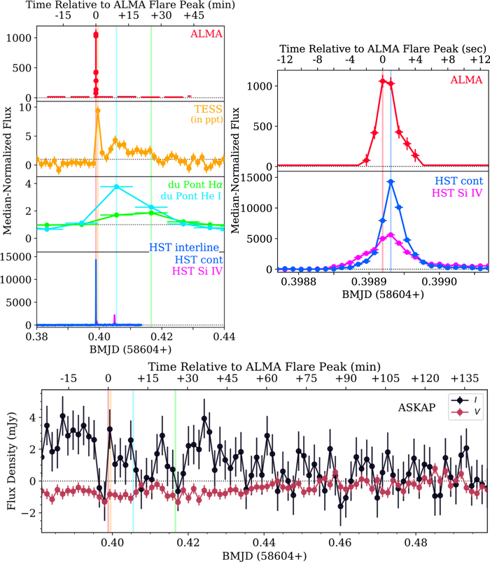
Figure 1. The complete light curve of the May 1 event at all wavelengths (left) and zoomed in to show the close correlation between millimeter and FUV as probed by ALMA and HST, respectively (right). Median-normalized flux is plotted to compare the relative brightening during the flare compared to quiescence as observed by all facilities. Vertical error bars indicate uncertainty in flux measurement, while horizontal error bars mark the time span of the individual observations from each telescope to aid the reader in interpreting potential emission delays between wavelength. ASKAP Stokes I and V light curves for the entire night of observations surrounding the flare are shown at the bottom. The colored vertical lines (red-ALMA, orange-TESS, blue-du Pont He I, green-du Pont Hα, purple-HST continuum, and magenta-HST Si IV) indicate the peak times of each facility to show correlation and delay. ALMA does not detect quiescent emission from Proxima Cen, so the line plotted outside of the flaring event indicates a 3σ upper limit on the quiescent flux.
Download figure:
Standard image High-resolution image2.1. Radio and Millimeter Wavelengths
The ASKAP observations show faint, ∼50% circularly polarized emission throughout the entire 14 hr observation, including a slowly declining flux component that is not seen on any other day of the campaign. The emission has an average flux density of 1.15 ± 0.14 mJy and −0.72 ± 0.09 mJy in Stokes I and V, respectively. We do not detect any radio burst counterpart. This apparent lack of correlation between low-frequency (<1 GHz) and higher-frequency activity is commonly observed from active M-dwarf stars (Kundu et al. 1988), and may indicate that the physical driver for low-frequency activity is independent of the processes driving flaring activity observed in higher-frequency wave bands.
As seen by ALMA (Figure 2, left), the May 1 flare reached a peak flux of 106 ± 7.9 mJy and luminosity of (2.14 ± 0.15) × 1014 erg s−1 Hz−1. The right panel of Figure 2 shows the ALMA light curve (top), along with the spectral index as a function of frequency (α, middle), and a lower limit on the fractional linear polarization (∣Q/I∣, bottom). This flare shows similar behavior to previous millimeter events (MacGregor et al. 2020). The light curve can be approximated by a Gaussian profile with a mostly symmetric rise and fall and no pronounced exponential tail. The spectral index becomes steeply negative at peak, while the fractional polarization is initially negative before flipping positive during the short decay. Outside of the flare and during the initial rise, the spectral index is consistent with emission from a quiescent stellar photosphere in the Rayleigh–Jeans regime. The change in both the spectral and polarization properties of Proxima Cen during this event indicate a change in the dominant emission mechanism from thermal blackbody to synchrotron or gyrosynchrotron emission.
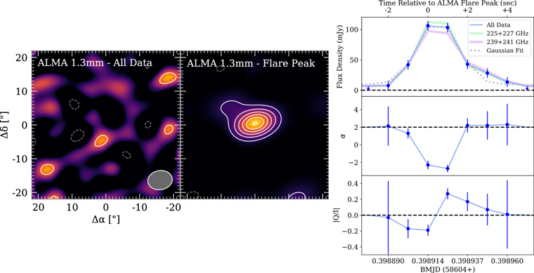
Figure 2. The >1000× brightness increase observed by ALMA during the flare is seen clearly by comparing an image of all ALMA data from May 1 (left) to the 1 s integration at the flare peak (center). Contours in both images are in steps of 2× the rms noise of 80 μJy and 7.9 mJy in the left and center images, respectively. The ellipse in the lower right corner of the left panel shows the synthesized beam. The spectral and polarization properties of the ALMA emission during this event are comparable to previously observed millimeter flares (right). At peak (shown in the light curve in the top panel), the spectral index as a function of frequency (middle panel, α, where Fν ∝ να ) becomes steeply negative while the lower limit on the fractional linear polarization (bottom panel, ∣Q/I∣) switches sign. A simple Gaussian fit (shown by the gray dotted line in the top panel) reproduces the overall shape of the light curve.
Download figure:
Standard image High-resolution image2.2. Optical Wavelengths
A bolometric energy of 1031.2 erg was measured by Vida et al. (2019) in TESS photometry for the initial May 1 event. TESS observed 71 other flares from Proxima Cen with comparable energies of 1030–1032 erg across 50 days of observations (Howard et al. 2018). Figure 3 shows the flare frequency distribution (FFD) for the energy (left) and amplitude (right) of flares from Proxima Cen as observed by TESS and Evryscope-South. Larger flares make up ∼75% of the combined sample (Howard et al. 2018), and these FFDs predict that flares with energies and amplitudes larger than the May 1 event occur once per day in the optical. The fact that the May 1 flare is apparently common in the optical yet extreme in the millimeter and FUV indicates that optical intensity does not necessarily scale to flare energies at other wavelengths and demonstrates the utility of multiwavelength coverage.

Figure 3. These flare frequency diagrams (FFD) show that this flare is relatively weak in the optical when compared against all other stellar flares observed from Proxima by Evryscope and TESS. We find flares of equal or greater energy (left) and amplitude (right) to the May 1 flare occur once per day in the optical. Evryscope observations included span 2016 January to 2018 August, while TESS observations span 2019 April to 2019 May. Flare energies are converted from each bandpass to bolometric energy as described in Section 2.2.
Download figure:
Standard image High-resolution imageEvryscope-South has monitored Proxima Cen with 2 minute cadence across 2 yr of observations (Ratzloff et al. 2019). Since TESS observed Proxima for less than one stellar rotation near Proxima's activity minimum (Wargelin et al. 2017), long-term flare monitoring with Evryscope provides a broader context to the flaring seen in the TESS data. We convert optical flare energies from the TESS and Evryscope bandpasses into bolometric energies using a ∼9000 K blackbody. This canonical temperature provides an approximate fit to the spectrum of typical flares (Osten & Wolk 2015). We also convert the TESS flare amplitudes into the Evryscope g' bandpass using an i-to-g scaling relation for flares from an M5.5 dwarf in Davenport et al. (2012). For the May 1 flare, these scaling relations yield an amplitude of 0.1 g' magnitudes.
We measure the cumulative FFD for the flare energy and amplitude by fitting a cumulative power law to the Evryscope and TESS flares in Figure 3. We calculate the uncertainty in the cumulative occurrence for each flare with a binomial 1σ confidence interval statistic, and estimate the uncertainty in our power-law fit through 1000 Monte Carlo posterior draws consistent with our uncertainties in occurrence rates. We measure an FFD for the bolometric energies E given by  , and an FFD for the g' amplitudes A given by
  . ν is the number of flares per day of an equal or greater size to E or A. Finally, because Evryscope has lower photometric precision than TESS, the smallest TESS flares are not always observed by Evryscope. We weight the flare rate of the smallest flares in the combined Evryscope and TESS FFDs by the TESS-only rates to remove bias from missing Evryscope flares.
Figure 4 (bottom left panel) shows the equivalent width curves over time for all of the emission lines we measured with du Pont during the May 1 flare. These emission lines display two types of behavior—He I, Hβ, Hδ, and H peak earlier, while Na D1 and D2, Ca H and K, Hα, and Hγ peak later. Delayed Ca K emission has been observed previously and interpreted as evidence for chromospheric evaporation through the Neupert effect (Kowalski et al. 2013). The Balmer lines increase substantially in width during the flare. Hα is double peaked throughout the event, and the Hβ line FWHM increases from ∼37 preflare to 45 km s−1 at peak.

Figure 4. A comparison (top) between the HST spectra before (blue) and during the flare (orange) show that several strong emission lines appear only during the flare. The equivalent width curves over time measured in the optical with du Pont (bottom left) show the dichotomy between lines that peak earlier and those that peak later, notably Ca K and Hα. The magnetic field strength in the radio-emitting source, B, can be constrained by the index of the accelerated particle distribution, δr , and the nonthermal energy in accelerated particles (lower right).
Download figure:
Standard image High-resolution image
2.3. Far-ultraviolet (FUV) Emission
The initial May 1 event exhibited an unprecedented rise in the star's pseudo-continuum FUV emission with an absolute FUV energy of 1030.3 erg, the largest ever recorded for Proxima Cen. M dwarf flares reaching nearly 1033 erg have been observed previously by HST from younger stars (Loyd et al. 2018b), and the equivalent duration of quiescent emission required to produce the same energy as the flare, 4300 s, is typical of daily UV flares on M dwarfs (Loyd et al. 2018a). The color temperature of the pseudo-continuum flare emission is 15,000–22,000 K, covering 0.002%–0.02% of the visible stellar hemisphere (5th–95th percentiles). A blackbody with these parameters would increase the flux in the TESS bandpass by only 0.07%–0.4%, meaning additional mechanisms are required to explain the 0.9% increase measured by TESS. FUV line emission increases by a smaller factor of only 100–5000× depending on the line, with broadening and asymmetric enhancements in redshifted emission out to 100 km s−1 typical of stellar FUV flares (e.g., Hawley et al. 2003; Loyd et al. 2018a). As seen in the top panel of Figure 4, several strong emission lines appear only during the flare, notably a singlet at 1247 Å and a quintuplet centered on 1299 Å that we have identified as originating from C2+ and Si2+ ions, respectively. In the second flare, the pseudo-continuum reaches only 450× the pre-flare level while the lines increase 1000×, which is more typical of FUV flares from M dwarfs (Loyd et al. 2018a).
3. Discussion
The multi-wavelength coverage of this extreme event yields relative energies and timings, allowing us to examine correlations between flare emission at different wavelengths. Only a few previous data sets include simultaneous FUV and optical coverage (e.g., Hawley et al. 2003), and these have largely shown a correlation between flaring emission at these wavelengths. The discrepancy between both the magnitude and timing of the optical emission compared with the millimeter and FUV emission that we see during the May 1 flare is new. The correlation between the millimeter and FUV emission suggests that these wavelengths both directly trace the initial "impulsive" phase that releases most of the flare's energy as electrons accelerate in magnetic loops. We interpret the emission at these wavelengths as arising from a hot blackbody with some contribution from synchrotron or gyrosynchrotron emission as indicated by the polarization signature at millimeter wavelengths. The delayed optical emission likely comes from heated plasma at the loop footpoints. Delayed optical line emission, specifically Hα, is commonly observed in solar flares (e.g., Benz 2017), with Hα emission peaking several minutes later during the "flash" phase, characterized by gentler energy release, possibly due to thermal conduction transport times (Canfield et al. 1990). The similar relative timing between wavelengths of the May 1 event sets up a strong parallel to solar flares.
3.1. Potential Emission Mechanisms
The spectral and polarization properties at millimeter wavelengths suggest that we are seeing the optically thin part of the gyrosynchrotron spectrum. We can infer the power-law index of nonthermal electrons, δ, from the the spectral index, α: α = 1.22 − 0.9δr (Dulk 1985; Güdel 2002; Osten et al. 2016). For the May 1 flare, this calculation yields δr = 3.9 ± 0.59, at the upper end of the range expected for hard radio spectra: 2.2 ≤ δr ≤ 3.9 (Dulk 1985). Following the method in Osten et al. (2016) and Smith et al. (2005), we assume a peak frequency of 50 GHz for the spectral energy distribution of gyrosynchrotron emission and calculate the integrated energy density in the flare over wavelength and time. This leads to a dependence of the total nonthermal energy on the index of the accelerated particle distribution, δr , and magnetic field strength in the radio-emitting source. Contours corresponding to the bolometric flare energy (1031.2 erg) and the FUV flare energy (1030.3 erg) are in red and blue, respectively, in Figure 4 (bottom right panel). A rough equipartition between nonthermal energy and the bolometric flare energy as observed by TESS (1031.2 erg) constrains the magnetic field strength to be between about 400–1500 G. Larger field strengths occur if the nonthermal energy is closer to the FUV flare energy of 1030.3 erg. Previous observations of Zeeman broadening in absorption lines of molecular FeH constrained the photospheric magnetic flux of Proxima Cen to be between 450–750 G (Reiners & Basri 2008), consistent with our estimate from these new ALMA observations. Interestingly, the spectral index of millimeter emission is the one characteristic of this event that differs significantly from solar flares. While the May 1 flare and all previous millimeter M dwarf flares exhibit steeply negative spectral indices with frequency, solar flares at millimeter wavelengths typically have positive indices (Krucker et al. 2013).
The extremely short duration of this event suggests that there is more to learn about the rapid time evolution of stellar and solar flares. Mouradian et al. (1983) discussed the possibility that complex flares are composed of many elementary eruptive phenomena (EEPs). Sequentially heated flare loops or "threads" form along an arcade structure, and combine or overlap to produce the total energy release of an event. The <10 s timescale of the initial May 1 burst roughly agrees with the duration of 10–20 s X-ray bursts observed in short cadence solar observations (Qiu et al. 2012). Notably, previous flares observed by ALMA at millimeter wavelengths all have short timescales, ranging from 2 to 35 s (MacGregor et al. 2020). Perhaps millimeter emission is a common part of stellar flaring, and often originates from these short burst-like events not commonly seen at other wavelengths.
3.2. Correlation between Millimeter and FUV Emission
Measuring the FUV and EUV radiation environment of exoplanets is critical to predicting and interpreting the chemical transformation and escape of their atmospheres (e.g., Ranjan et al. 2017; Owen 2019). However, observations at these wavelengths can only be performed from space and are limited by the dearth of facilities and absorption in the intervening interstellar medium. These are the first simultaneous millimeter and FUV observations of a stellar flare and are therefore the first to show a strong correlation between emission at these wavelengths. Notably, some previous observations have shown a correlation between microwave and hard X-ray emission during solar flares (Wiehl et al. 1985).
If this trend is representative of flares in general, we can use the peak luminosity at millimeter wavelengths (2.14 × 10¹³ erg s−1 Hz−1) and in the Si IV lines at 1393 and 1402 Å (5.41 × 1027 erg s−1) to estimate the associated FUV luminosity for the millimeter flares previously observed with ALMA without simultaneous HST observations. We accomplish this by deriving a scaling factor from the millimeter to Si IV (FUV) luminosity and applying it to previously millimeter measurements. For the 2017 Proxima Cen flare (MacGregor et al. 2018), the associated FUV luminosity might have been 5.1 × 1027 erg s−1, while the previous largest AU Mic flare (MacGregor et al. 2020) might have had an FUV luminosity of 4.9 × 1028 erg s−1. This prediction is consistent with previous HST observations of flares from AU Mic, which had luminosities of 1.8–3.2 × 1028 erg s−1 (Loyd et al. 2018a). It is striking that the FUV luminosity for the Proxima Cen and AU Mic events are within an order of magnitude of each other given the significant age and spectral type—4.85 Gyr, M5.5 (Kervella et al. 2003), and 22 Myr, M1 (Mamajek & Bell 2014), respectively—difference between the two stars. If millimeter emission can serve as a proxy for FUV emission from stellar flares, we will have a powerful new tool to determine stellar FUV emission, required input for models of planetary atmosphere evolution and abiotic oxygen accumulation (Luger & Barnes 2015).
4. Conclusions
The observations of this one event observed by multiple facilities at millimeter to FUV wavelengths already challenges our current theoretical models of stellar flaring. Proxima Cen is a unique target given that it hosts a planet in the habitable zone but also produces anomalously powerful flares for its old age. Can a planet truly be habitable in this environment? It is clear that necessary pieces are missing from our current understanding of M dwarf flares in order to answer that question. We expect to learn much more as we synthesize the available data from this project and from future flare campaigns. This paper presents the results from just a few minutes of the available data. Many other flaring events are detected simultaneously across multiple facilities (including ALMA and HST) during the full 40 hr campaign. If the correlation between FUV and millimeter flaring emission holds, there is potential for future all-sky millimeter surveys (e.g., the Atacama Cosmology Telescope; Naess et al. 2020) to be able to provide constraints on the high-energy radiation environment of exoplanet host stars and inform discussion of planetary habitability.
This paper makes use of the following ALMA data: ADS/JAO.ALMA #2018.1.00470.S. ALMA is a partnership of ESO (representing its member states), NSF (USA) and NINS (Japan), together with NRC (Canada) and NSC and ASIAA (Taiwan), in cooperation with the Republic of Chile. The Joint ALMA Observatory is operated by ESO, AUI/NRAO, and NAOJ. This research is based on observations made with the NASA/ESA Hubble Space Telescope obtained from the Space Telescope Science Institute, which is operated by the Association of Universities for Research in Astronomy, Inc., under NASA contract NAS 526555. These observations are associated with program 15651. This paper includes data collected by the TESS mission. Funding for the TESS mission is provided by the NASA Explorer Program. The du Pont Telescope observations benefited from the assistance of Nidia Morrell and the staff of Las Campanas Observatory.
M.A.M. acknowledges support for part of this research from a National Science Foundation Astronomy and Astrophysics Postdoctoral Fellowship under Award No. AST-1701406. M.A.M. and A.J.W. acknowledge support from NRAO Student Observing Support (SOS) grants SOSPA6-011 and SOSPA6-021. Support for HST program number 15651 was provided by NASA through a grant from the Space Telescope Science Institute, which is operated by the Association of Universities for Research in Astronomy, Incorporated, under NASA contract NAS5-26555. T.B. acknowledges support from the GSFC Sellers Exoplanet Environments Collaboration (SEEC), which is funded in part by the NASA Planetary Science Divisions Internal Scientist Funding Model.
Software: CASA (v5.3.0 & v5.11.0 McMullin et al. 2007), IRAF (Tody 1986, 1993), Lightkurve (Lightkurve Collaboration et al. 2018), astropy (Astropy Collaboration et al. 2013, 2018), astroquery (Ginsburg et al. 2019).
Appendix
Details on how the data were obtained, reduced, and analyzed are provided below for all facilities involved in the multiwavelength campaign. The wavelength range and exposure times for each instrument are listed in Table 1. All observing times are reported in UTC and Modified Barycentric Julian Date (MBJD). We have chosen to apply a barycentric correction, which accounts for differences in the Earth's position with respect to the barycenter of the solar system, due to the wide spread in location between the ground- and space-based facilities involved.
Table 1. Details of Multiwavelength Observing Campaign
| Facility | Center | Wavelength | Avg. Integration |
|---|---|---|---|
| Wavelength | Range | Time (s) | |
| ASKAP | 33.8 cm | 29.0–40.3 cm | 10 |
| ALMA | 1.29 mm | 1.24–1.34 mm | 1 |
| TESS | 775 nm | 580–970 nm | 120 |
| du Pont | 6675 Å | 3500–9850 Å | 800 |
| HST | 1435 Å | 1160–1710 Å | 1 |
Download table as: ASCIITypeset image
A1. ASKAP
We observed Proxima Cen with ASKAP (McConnell et al. 2016) on 2019 May 1 09:01 UTC (scheduling block 8604) using a single on-axis (boresight) beam. We took the observation at a central frequency of 888 MHz (33.8 cm) with 288 MHz bandwidth, 1 MHz channels, and 10 s integrations, lasting 14 hr in total. The primary calibrator PKS B1934−638 was observed for 31 minutes immediately after the Proxima Cen observation (scheduling block 8606). We used on-dish calibrators to calibrate the frequency-dependent XY-phase.
We processed the ASKAP observations using the Common Astronomy Software Applications (CASA) package version 5.3.0 (McMullin et al. 2007). We determined flux scale, bandpass, and polarization leakage calibration using the observation of PKS B1934−638. We used basic flagging routines to remove radio-frequency interference that corrupted approximately 20% of the data.
We imaged the Proxima Cen field using the task tclean with a Briggs weighting and robustness of 0.0, using 6000 × 6000 pixels to include the full primary beam and the secondary sidelobes. We deconvolved the image using the mtmfs algorithm with a cell size of 25 and scale sizes of 0, 5, 15, 50, and 150 pixels. These imaging parameters enabled us to account for bright, complex field sources present both within and beyond the primary beam. To model sources with nonflat spectra, we used multifrequency synthesis with two Taylor terms. We excluded a  square region centered on Proxima Cen from deconvolution to allow modeling of field sources without removing temporal and spectral variability of Proxima Cen. We deconvolved to a residual of 3 mJy beam −1 to minimize PSF side-lobe confusion at the location of Proxima Cen. After deconvolution, we subtracted the derived field model from the calibrated visibilities using the task uvsub, and vector-averaged visibilities across all baselines longer than 200 m for each instrumental polarization.
Using the vector-averaged visibilities, we formed dynamic spectra for the four Stokes parameters (I, Q, U, and V) consistent with the IAU convention of polarization, following Zic et al. (2019). To improve the signal-to-noise ratio in the dynamic spectra, we averaged over a factor of 24 in time and 16 in frequency, giving a dynamic spectrum resolution of 240 s and 16 MHz. We determined the rms noise in the dynamic spectra by taking the standard deviation of the imaginary part of the visibilities for each Stokes parameter, finding 3.4 mJy, 1.3 mJy, 1.5 mJy, and 1.0 mJy for Stokes I, Q, U, and V, respectively. We formed light curves by averaging the dynamic spectra across frequency. The typical rms uncertainty in the light curves for Stokes I, Q, U, and V is 0.89 mJy, 0.36 mJy, 0.38 mJy, and 0.23 mJy. The higher level of rms noise in Stokes I products arise from imperfect subtraction of field sources, leading to enhanced levels of sidelobe confusion at the location of Proxima Cen.
To validate our visibility-domain approach to constructing light curves, we imaged the Proxima Cen field in Stokes I and V at 4 minute intervals, measuring the peak flux density at the location of Proxima Cen. We found that the resulting light-curves agreed well with those from the visibility-based approach.
A2. ALMA
The Atacama Compact Array (ACA) of ALMA observed Proxima Cen from 04:08:17 to 10:13:04 UTC on 2019 May 1 in four scheduling blocks (SBs) that each lasted approximately 93 minutes. During each SB, Proxima Cen was observed in 6.5 minute integrations or "scans" alternating with a phase calibrator, J1424-6807, for a total of roughly 49 minutes on-source. The flare discussed in this paper occurred during the final SB. There were nine antennas in the ACA during these observations spanning baselines of 10–47 m. Flux and bandpass calibration were performed using the bright quasar J1337-1257.
For these observations, the correlator was set up to maximize continuum sensitivity. Four spectral windows were centered at 225, 227, 239, and 241 GHz, with a total bandwidth of 2 GHz each, for a combined bandwidth of 8 GHz. Two linear polarizations (XX and YY) were also obtained. The raw ALMA data were reduced in CASA version 5.1.1 (McMullin et al. 2007) using the ALMA pipeline. Deconvolution and imaging was performed using the clean task in CASA.
We can use the broad bandwidth and dual polarization of these ALMA observations to determine both the spectral index as a function of frequency (α, where Fν ∝ να ) and a lower limit on the fractional linear polarization (∣Q/I∣) during the large flare on May 1. We note that since we do not constrain Stokes U with these observations, ∣Q/I∣ is only a lower limit to the true linear polarization fraction  . In order to calculate the spectral index of the flaring emission, we fit independent point-source models to the millimeter visibilities from both the lower and upper sidebands. At peak, the flux densities are 112 ± 10.4 mJy and 97.6 ± 11.0 mJy for the lower and upper sidebands, respectively, yielding a spectral index of α = −2.29 ± 0.48. We checked the accuracy of the frequency-dependent amplitude calibration performed by the ALMA pipeline by comparing the results for the flux, bandpass, and phase calibration sources to the ALMA calibrator catalog (Bonato et al. 2018). To determine a lower limit on the fractional linear polarization, we fit point-source models to the XX and YY visibilities independently and compute the Stokes
  and
and  , where EX and EY are antenna voltage patterns. This process yields ∣Q/I∣ = −0.19 ± 0.07 at flare peak.
A3. TESS
TESS is equipped with four cameras that each cover one 24 × 24 degree field of view and have an approximate effective aperture size of 10 cm. The throughput of TESS is optimized for the red-optical, with >50% throughput at 580–970 nm. TESS is in a high Earth orbit, with an average orbital period of 13.7 days. The four TESS cameras are aligned to project onto the sky in a 1 × 4 grid and the field of view is adjusted every two orbits. TESS integrates continually using frame transfer CCDs, which are read out every 2 s. The full 96 × 24 degree field of view is stored by the spacecraft every 30 minutes, while select targets are stored at a high cadence of 2 minutes. These 2 minute cadence observation represent an integration time of 96 s, because 20% of data is rejected by the on-board cosmic-ray mitigation algorithm. Proxima Cen was observed by TESS at 2 minute cadence from 2019 April 22 to 2019 June 19, covering two observing sectors (Sectors 11 and 12). The May 1 flare occurred during Sector 11.
We analyzed the TESS data starting with calibrated pixel-level data rather than calibrated light-curves because the TESS systematic removal is not designed to handle impulsive outliers, such as flares. We used the Lightkurve software package (Lightkurve Collaboration et al. 2018) and dependencies astropy (Astropy Collaboration et al. 2013, 2018) and astroquery (Ginsburg et al. 2019) to download the data from the Mikulski Archive for Space Telescopes (MAST) archive, and to extract a light curve from the pixel-data. We used the "threshold" method to determine the pixel mask used to create the light curve, with the threshold set at 3σ. We removed instrumental systematics using the Pixel Level Decorrelation (PLD) algorithm (Deming et al. 2015; Luger et al. 2016) implemented in Lightkurve.
We took care to explore the impact of including different pixels in both the light curve extraction aperture and in the PLD analysis region on the May 1 flare. While the May 1 flare was clearly detected by TESS, the exact shape of the flare is somewhat challenging to resolve because of the relatively low signal-to-noise detection of the flare and its short duration relative to the TESS sampling cadence. We found that the primary peak of the flare (this is the time period that overlaps with the ALMA flare) was insensitive to changes in the pixels used in the analysis but the flux in the shape of the decay phase of the flare, the second and third peaks in the TESS data, were susceptible to being over fit by the PLD algorithm. We chose a set of pixels so that the PLD model did not have strong variability during the flare, as this likely represents a solution that is not subject to overfitting.
A4. du Pont Telescope
The Echelle Spectrograph on the 2.5 m Iréné du Pont Telescope at Las Campanas Observatory provides complete wavelength coverage from ∼3500 to 9850 Å at a resolution of ∼40,000 in a 1'' slit. The weather was clear and seeing ∼09. Exposures were taken starting at 04:30 UT and continuing until 10:39 UT with the only gaps caused by readout of the CCD. Exposure times ranged from 600 to 900 s during the flare, with shorter exposures taken during the peak because the S/N on the emission lines was noticeably higher. ThAr lamp spectra were taken at the beginning and end of the sequence.
IRAF (Tody 1986, 1993) tasks were used for the data reduction from the 2D CCD images through extraction and wavelength calibration. Basic CCD reduction began with overscan subtraction, flat-fielding, and bad pixel correction. The flat field was made by averaging together 52 flats taken between April 25 and May 6. Each flat is a daytime sky spectrum taken through a diffusing glass and then divided by a 15 × 15 pixel box-car filtered version of itself. Spectra were extracted with the apall package. For orders in which the continuum was traceable, each extraction aperture was recentered on each order. For orders at λ < 4400 Å that had bright emission lines, but little continuum, the apertures were centered based on the emission line position. Background regions were set individually for each order. The extraction was variance weighted. Wavelength calibration was based on only the ThAr lamp taken at the end of the night, i.e., at 10:48 UT.
Using a custom IDL code, we fit the continuum with a third-order polynomial and subtracted it. Also with a custom code, we measured the equivalent widths of the Hydrogen Balmer series (Hα through H), Ca H and K, He I, and Na I D1 and D2 lines. Integration limits were set by visual inspection of each spectrum. The per pixel uncertainty was estimated from the noise in the continuum on either side of the line and then propagated into an uncertainty on the equivalent width.
Six spectra cover the start of the flare through the end of the night (Table 2). The spectrum containing the UV flare started exposing at 09:13:38 UT and had an exposure time of 900 s. The first exposure with substantial flare emission started at 09:29:40 UT and also had an exposure time of 900 s.
Table 2. Observing Log for du Pont Echelle
| Exposure Start | Exposure Middle | Exposure Time |
|---|---|---|
| (UT) | (MJD—2,458,604) | (s) |
| 09:13:38 | 0.894369 | 900 |
| 09:29:40 | 0.905503 | 900 |
| 09:45:41 | 0.916626 | 900 |
| 10:01:43 | 0.926893 | 750 |
| 10:15:14 | 0.935411 | 600 |
| 10:26:16 | 0.943942 | 750 |
Download table as: ASCIITypeset image
A5. HST
We collected the HST data using the Space Telescope Imaging Spectrograph (STIS) instrument with the E140M grating. The data are in time-tag format, meaning STIS operated as a photon counting detector. The spectral resolving power of the instrument is R = λ/Δλ = 45,800 and time resolution is, in practice, limited by signal-to-noise rather than the instrumental resolution. Greater time resolution is possible in spectral and temporal ranges with greater flux. The intrinsic time-tagging of the MAMA detector is 125 microseconds.
We obtained the reduced HST data products from the MAST archive on 2019 November 8. We then used a custom code to calibrate the wavelength and apply effective-area weighting to photons in the raw time-tag ("_tag.x1d") data files. The code extracted events from regions on the detector where the spectral traces of the Echelle fall, then used regions without signal above and below the spectral trace to estimate and subtract a background count rate. In this way, it generated time-integrated spectra that it then compared to the fully pipeline-reduced spectra to estimate the photon wavelengths and effective-area weights, producing a calibrated photon list. From the calibrated photon lists, we integrated photons with arbitrary wavelength and time binning to generate light curves of emission from specific wavelengths and spectra of emission integrated over intra-exposure time ranges. This is the same process used by Loyd et al. (2018a, 2018b). Using our custom code avoided background oversubtraction issues that appeared when generating subexposure spectra with the HST CALSTIS tools.