In a previous post I demonstrated how one can assign customers to the nearest warehouse using a well-known clustering algorithm. In this post I will demonstrate how a single warehouse location problem can be approached by applying center of mass calculation in R. The idea is to locate the warehouse in right in the average center of demand, taking into account spatial distribution of customer demand.
Below, I define the center of mass function. It takes into account x and y coordinates. I.e. we simplify the problem by neglecting the vertical z-axis of our spatial location problem. w stands for the weights of the respective coordinates. This could e.g. be the demand by location.
center_of_mass <- function(x,y,w){
  c(crossprod(x,w)/sum(w),crossprod(y,w)/sum(w))
}
Next, I create a dataframe representing customer demand. I apply latitude and longitude coordinates. Latitude value range is from -90 to +90. Longitude value range is from -180 to +180. I create 40 customers with random location and demand, somewhere within the coordinate-system.
customer_df <- as.data.frame(matrix(nrow=40,ncol=3))
colnames(customer_df) <- c("lat","long","demand")

customer_df$lat <- runif(n=40,min=-90,max=90)
customer_df$long <- runif(n=40,min=-180,max=180)
customer_df$demand <- sample(x=1:100,size=40,replace=TRUE)
Below I print the header of that dataframe:
head(customer_df)## lat long demand
## 1 -46.40781 43.13533 4
## 2 -29.06806 98.97764 72
## 3 -75.84997 127.47619 44
## 4 -54.37377 55.16857 66
## 5 71.67371 178.98597 21
## 6 -34.03587 -42.88747 100Using that dataset I can calculate the center of mass:
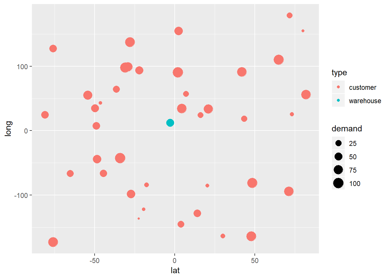
center_of_mass(customer_df$lat,customer_df$long,customer_df$demand)## [1] -2.80068 12.49750To assess this result, I plot the customer demand using ggplot2:
library(ggplot2)
joint_df <- rbind(customer_df,c(center_of_mass(customer_df$lat,customer_df$long,customer_df$demand),50))
joint_df$type <- c(rep(x="customer",times=40),"warehouse")
ggplot(data=joint_df) + geom_point(mapping=aes(x=lat,y=long,size=demand,color=type))
The center of mass method can be well combined with heatmap visualisation of spatial customer demand distribution. For this, you can read my blog post on how to create heatmaps in R, using the Leaflet package: Leaflet heatmaps in R
I also use other packages to visualize spatial distribution of customer demand, including deckgl: Using deckgl in R for spatial data visualisation

Data scientist focusing on simulation, optimization and modeling in R, SQL, VBA and Python


7 comments
Hi Linnart,
While this is very useful, I was wondering could you also show how would we calculate the same using optimization (like as Excel Solver) but via R only.
I understand that the difference would be small but I was just curious if it is possible to do that with R.
Again thanks for this.
Modeling this as a mathematical program is pretty straight forward. You need an objective, which is the euclidean distance between all customers or suppliers to the chosen warehouse location. The optimization variables are the coordinates of the warehouse location.
Thanks Linnart. To be honest, I do not know how to run even a fairly simple optimization using R.
However, I did find another useful package in R called “Gmedian” which finds the centre of minimum distance, only drawback is that it does not consider demand.
However, that can be theoretically overcome by creating demand no. of multiples/copies of each customer, not sure how practical it would be though.
Thanks again. Your content is very useful and informative.
Hi Ibrahim.
You can use lpSolve in R. You can send me the data and can develop a template for you that fits your problem and data. Should only take 1-2 consultation hours. If interested let me know and contact me via the contact form or via LinkedIn.
Regarding geometric median, which you have pointed out, it is true that it will result in a different solution compared to center of mass. But, the center of mass can be calculated easily and at very low cost. The geometric median can only be derived numerically. And this means, the cost is higher. Also, the center of mass and the geometric median are both based on strong assumptions and are so to say both “wrong”. They are, however, good enough when used in the right context.
The center of mass is the center of a heatmap, when e.g. visualizing demand or supply distribution spatially. It is easy to understand and can be a good start point for searching the optimal location of e.g. a warehouse. But, it is only a start point. The cost optimum depends on many more complex factors. Examples:
– parcel shipment costs are zone based, not linear as assumed by e.g. center of mass calculation
– sea freight costs FCL and LCL depend mostly on the port, not on the distance
– air freight depends much on the airport too
– intermodal freight depends mostly on the availability of rail connections (rail is cheaper than trucking)
– labour costs depend on the region / country
– availbility of warehouse facilities for rent, and the cost of renting them depends very much on the region as well
This is why focusing too much on e.g. a geometric median vs. center of mass discussion is the wrong approach. Do not worry too much about whether you choose geometric median or center of mass. Pick one of them and get started. Focus more on the additional factors that I listed abov.
Hi Linnart –
Thanks for sharing this problem.
I really like how this solution weights the result by demand, however, how does the R code change if I want to calculate the distances taking the curvature of the earth into account?
Thanks
Hi MSG.
Thank you for your question. I get this question a lot, and maybe when I got the time I will write another blog post on this topic comparing various approaches. I should also make a online course or something on this topic.
To your question: No, this is just the 2D euclidean distance. If you want to be mathematically totally correct, you can do the following:
1) Use the distHaversine() function from the geosphere package in R to calculate non-Euclidean distance
2) Using that distance calculate the geometric median, not the arithmetic median
But my point is it is really up to you to choose what is the EASIEST to implement and to COMMUNICATE. Because, if you do above exercise, you will quickly find that the “optimal” location indicated by the calculation differs only marginally. And in the end, what are we really looking for? We are looking for a warehouse location that minimizes total cost and lead time.
It is important to remember that this is not a mathematical exercise, it is a business exercise. In the end our shipping costs will depend on our freight rate agreements. For CEP (course, express, parcel) we will usually be charged on a “rate zone” basis, and for inbound freight transported by intermodal transport our transport costs will depend more on the proximity to a “good” port with good sea freight rates and good rail connections. This is why Atlanta for example is a very good logistics hub.
My point is: Don’t get lost in mathematical thinking. In my opinion this exercise is only to get a rough estimate of where a good warehouse location might be. You then have to define candidate locations and run cost simulations and lead time simulations for these candidates. That will be the most practical and reliable approach. You can off course also define a comprehensive mathematical model from the start, that e.g. takes into consideration the freight types and their rate structure (for CEP e.g. zone based rates). But if you also do milk-runs or similar, then this will quickly become an expensive exercise.