All Our Electricity Generation Is Weather Dependent

July 17, 2023

The OpenNEM website gives access to several ways of viewing Australia’s electricity usage.  One I like shows Flexibilty.  Figure 1 shows plots for the week to Tuesday 11th July of consumption sourced from Variable (wind and solar), Fast Flexible (gas, hydro, diesel, battery), and Slow Flexible (black coal and brown coal). I chose this period because it includes Tuesday 4th, Friday 7th and Saturday 8th, and illustrates just how variable the Variables can be.

Figure 1: Screenshot of Flexibilty, NEM

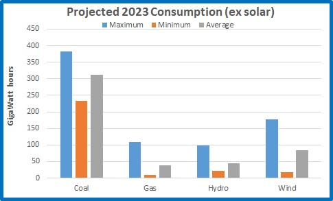
Obviously, when Variables are high Flexibles are low and vice versa.  Notice that Variables have one peak at noon each day, as solar generation far exceeds wind- in daylight hours, but Flexibles have two peaks each day, morning and evening.  Figure 2 is my plot for the first week of July, combining all non-variables and showing the total consumption:

Figure 2:  Total Consumption 1-7 July 2023

The total (red) shows the two peaks, morning and evening, and the overnight dip to baseload at about 20,000 MW.  Note that variable generation (green) has a midday peak due to solar that rapidly descends with the sun to a night time level far below baseload.

Note also that on the evenings of the 3rd and 4th total consumption is made up almost entirely of flexible generation- variable was only 3.4% of the total on the 3rd and 3.9% on the 4th.

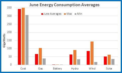
The next figures contrast conditions on the best day of the week for variables with those on the worst day.

Figure 3:  4th July Consumption- Worst for Variables

Monday and Tuesday, the 3rd and 4th, saw extensive cloud cover and rain over much of eastern Australia, especially Queensland, while winds were very light in the south. This was the worst day for wind and solar, peaking at about 6,000 MW at 12.30, dropping to 1,170 MW at 6 pm.  Conversely, it was the best day for coal generators who could maintain steady generation all day.  Contrast this with the 7th:

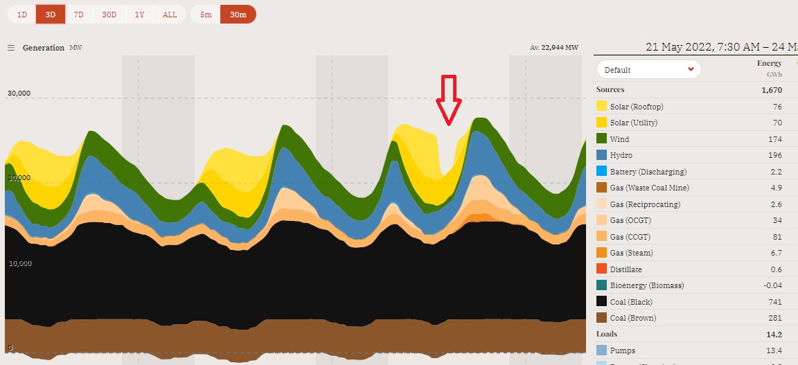
Figure 4:  7th July Consumption- Best Day for Variables

The sun was out and the wind was fair. This was a great day for wind and solar, producing 60% of all electricity needed in the middle of the day.  Note how coal fired generators had to decrease then increase very rapidly (nearly 80% increase from 3 pm to 6.30 pm).  That’s not how they were designed to operate.

Electricity statistics for the first week of July show how thoroughly weather-dependent are wind and solar. However, they also show the resilience of non-variable generation, and show the excellent Capacity Factor that coal can achieve.  Capacity Factor is the actual generation as a percentage of nameplate capacity.

Figure 5:  Coal generation Capacity Factor 1 -7 July 2023

Even with Callide C out of action until next year, coal’s capacity factor dropped below 50% only on the 8th.  It peaked at over 80% on every day of the weak, averaged 73.6% and reached 90% on the 4th.  While wind’s capacity factor was at 94% on the evening of the 7th, at 5.30 pm on the 3rd it was only 9.7%, and at that same time solar capacity factor was practically zero.

Thank goodness for variable generation, which adjusts to the vagaries of wind and solar.  In Australia, even fossil fuelled electricity is dependent on the weather.

In my next post I will show why you shouldn’t expect batteries and hydro dams to come to the rescue anytime soon.

(Source: OpenNEM)

Analysis of Parallel Tmax Data from Brisbane Aero

May 30, 2023

Dr Jennifer Marohasy has recently stirred up the Bureau of Meteorology and their usual uncritical apologists with her analysis of three years of parallel data obtained for Brisbane Airport (after years of denial and obstruction by the BOM).  This relates to side-by-side recording of temperatures taken from the traditional mercury Liquid In Glass (LIG) thermometer and the repacement Automatic Weather Station (AWS) which show that “41% of the time the (AWS) probe is recording hotter than the mercury, and 26% of the time cooler.

She also identified a step change in AWS values in December 2019 which she thought represented recalibration of the AWS system.  The BOM denied this, “explaining there was a fault in the automatic weather station that was immediately fixed and operating within specifications from January 2020 onwards.”

This post is a further analysis of the parallel data (kindly shared by Dr Marohasy).  It shows that:-

  • The discontinuity in December 2019 is beyond doubt.
  • There was indeed a fault in the AWS in December 2019, but the repair resulted in the “fixed” AWS reading on average 0.23 degree Celsius higher than it was before the fix (for equivalent LIG temperatures) for the next two and a half years.
  • Before the AWS was “fixed” it was recording temperatures on average 0.2C cooler than the LIG.  After the “fix”, the AWS was on average less than 0.1C warmer.
  • Before the “fix”, 3.6% of the AWS recordings were higher than the LIG on the same day, and 86.2% were lower.
  • After the “fix”, 47 % of the AWS recordings were higher than the LIG on the same day, and 16.5% were lower.
  • 26.7% of all readings before and after the “fix”were outside of the +/- 0.1C range.
  • There were seasonal variations in the difference between AWS and LIG.
  • Unexplained spikes continued randomly before and after the AWS was “fixed”.
  • The “fixed” AWS may have begun to deteriorate again in mid-2022.

In analysing the parallel data I compared same day observations by calculating the difference between AWS and LIG readings.  Figure 1 shows daily differences in degrees Celsius as a time series.

Fig. 1: Daily differences (outliers removed)

A 31 day running mean is a good way to see changing patterns:

Fig 2: 31 day running average of differences

There was a sharp dip and sudden rise in values in December 2019 to above zero difference, at the time of the AWS fault and repair.  Note the dip below zero in June and July 2022.

Figure 3 shows the daily differences from 31 July 2019 until the “fix”.

Fig. 3: Daily values to 22/12/19.  Note large fluctuations from 16thDecember:

I excluded values from 16th to 22nd December when the AWS was faulty.

BOM experts have repeatedly claimed that AWS systems report temperatures that are predominantly within +/- 0.1C of LIG readings.  From 31/7/19 to 15/12/19 there were 80 incidences (58%) of the difference of AWS minus LIG being less than -0.1C and 2 incidences (1.45%) of the difference being greater than +0.1C.  From 23/12/19 to 30/7/22 there were 30 incidences (3.2%) of difference < -0.1C and 178 incidences (18.8%) of difference > +0.1C.  26.7% of all readings before and after the “fix”were outside of the +/- 0.1C range.

The following plots analyse the data for differences outside this range.

Fig. 4:  Running count of days with difference more than +0.1C

The number of days with AWS reading more than +0.1C above LIG rose steadily from 23 December.

Fig. 5:  Running count of days with difference below -0.1C

The break in December 2019 is obvious.

A 31 day running count is a good way to see changing patterns:

Fig. 6:  31 day count of days with difference more than +0.1C

Before the AWS “fix”, differences over 0.1C were rare.  After this, the number immediately increased.  Note that the incidence of days with a difference over 0.1C fluctuated in large swings.  In early December 2020, 17 out of the previous 31 AWS readings were more than +0.1C higher than LIG, and in October 2021 there were 16.  The count continued fluctuating while gradually decreasing, with a drop to zero in early and mid-2022.  This may indicate a deterioration in the AWS system.

The fluctuations are also seen in differences below -0.1C.

Fig. 7:  31 day count of days with difference lower than -0.1C

There was clearly a discontinuity in December 2019, followed by fluctuations in the incidence.

Is there a pattern in the months after the AWS was “fixed”?

The next figures plot 31 day counts by month of the year from January 2020.

Fig. 8: Count of differences >+0.1C by month

Higher frequency of differences > +0.1C occur in early winter and summer.  Lower counts occur in March, April, July, and August.

Fig. 9: Count of differences <-0.1C by month

Note that there is a clear seasonal pattern: most differences occur in July; least from October to January.

Figures 10 and 11 are timeseries of monthly counts.

Fig. 10:  31 day counts of differences > +0.1C each month

The swings we saw in Figure 6 above are replicated with months more easily identified.  There were spring peaks in 2020 and 2021, but there was also a peak in May and June of 2020.  Differences were low from December 2021 to July 2022.  Was the AWS beginning to malfunction?

Fig. 11:  31 day counts of differences under -0.1C each month

This is (almost) the opposite of Figure 10.  There are more days with AWS less than LIG in winter months.  However winter of 2022 saw an unusually high number of days with AWS cooler than LIG.  In July 2022 up to 42% of AWS readings were more than -0.1C different from LIG. 

The next two plots show the frequency (as a percentage) of all differences before and after the “fix”.

Fig. 12: Frequency of differences between AWS and LIG: to 15/12/19

From 31/7/2019 to 15/12/2019 AWS was on average 1.7C cooler than the LIG, as shown. 

Fig. 13: Frequency of differences between AWS and LIG: from 23/12/19

The plot of difference values has shifted right.  The BOM is correct in that 75% of AWS readings after the “fix” were within +/- 0.1C of LIG, but the average difference increased from -0.17C to +0.05C: about +0.2C. 

Also, the range of differences remained large.

Fig. 14: Differences each month before and after the AWS was “fixed”

Apart from the circled values in December 2019 when the AWS was faulty, the range of differences between AWS and LIG was similar after the “fix”.   Spiles were even greater.

Greatest difference to 15/12/19:               +0.6C

Smallest difference to 15/12/19:               -0.5C

Greatest difference from 23/12/19:          +0.7C

Smallest difference from 23/12/19:          -0.7C

AWS values from 31/7/2019 to 30/7/2022 show a clear discontinuity in December 2019, but the AWS continued to “spike” above and below LIG values.  The only change was that the AWS was now reading about 0.2C warmer than before.    Figures 15 and 16 show this in a different way.

Fig. 15: Daily AWS values before and after the “fix” for corresponding LIG values

They are very close, but different.

Fig. 16: Zooming in: Daily AWS values before and after the “fix” for corresponding LIG values

The trendlines of the two plots are offset, and the difference is about 0.2C, as shown above.

In conclusion:

My analysis confirms that Dr Marohasy is correct: the AWS system at Brisbane Aero reads higher than the LIG thermometer, and there was a distinct step up after the AWS was “fixed” in December 2019.

The Bureau of Meteorology cannot claim there was no difference following December 2019.  One of the two records is accurate, the other is not.  If the AWS system was performing within specifications after 23/12/2019, it was definitely not before then.

One Minute Data and Extremes Part 1: Thangool

May 23, 2023

In 2017 I purchased from the Bureau of Meteorology (BOM) a slab of one minute data from 16 country Queensland stations with Automatic Weather Stations (AWS).  One minute data is the temperature of the final second of every minute- 1,440 of them each day.  I posted a few times about this, and now I return to it to check on some recent claims by the BOM.

They repeatedly assert that the difference between AWS temperatures and those measured by mercury thermometers (LIG) is less than 0.1 degree Celsius.

The one minute data, infuriatingly, is NOT published by the BOM for more than 72 hours, and is NOT used for any daily temperature recording.  The AWS reads the temperature every second in each minute, but only the highest, lowest and final second temperatures are kept.  The highest of those highest one second values, from 9:00 a.m. to 8:59 a.m. next day, becomes the maximum (Tmax) of the day, and the lowest (also 9:00 a.m. to 8:59 p.m.) becomes the minimum (Tmin).  Tmax and Tmin are freely available, published at Climate Data Online (CDO).  One minute data is available at a cost, and at the time of my purchase did not include one minute high and low values.  Therefore, I can only compare daily data for final seconds of 1,440 minutes with the one highest and one lowest seconds, and can only estimate their time of recording.  Grrr!

A further source of frustration is that daily temperatures at CDO for many places have not passed Quality Assurance checks more than six years later- but that doesn’t stop them from calculating monthly means for them, claiming the monthly means are quality controlled.

Therefore in this series of analyses I only use daily data that is quality controlled.

Thangool is a very small town about 120km south-west of Gladstone and has the airport for Biloela.   Figure 1 shows the difference of the daily Tmin (one second value) minus the lowest one minute (final one second value) for February 2017.

Figure 1:  Daily Minimum Difference

Note that no daily minimum value is more than 0.1C below the lowest one minute value on any day in February.  No apparent issue there.

Figure 2:  Daily Maximum Difference

Clearly the difference is greater for maximum temperatures.  On 11 out of 28 days (39.3%) the difference between the maximum temperature and the highest temperature in the final second of any minute was greater than +0.1C.  The greatest difference was on 19 February when Tmax was +0.7C higher.  And that is at least, as I will show.

That is not comparing AWS readings with the old mercury LIG thermometers- we need parallel data for that, which the BOM is extremely reluctant to release.

However, we can draw some inferences.

Figure 3 is a plot of 1-minute temperature at Thangool Airport between 11:00 a.m. and 2:00 p.m.  on 19 February 2017 as measured by the AWS, the maximum recorded by the AWS, and an illustration of what an LIG thermometer might have recorded.  If we assume the AWS accurately simulates a mercury thermometer, I have shown how the mercury would have risen in steps: it would not have fallen after these steps until reset at 9:00 a.m. next day.  The maximum was reached after 1:00 p.m. and was recorded by the AWS as 35.7C.

Figure 3: One minute and Maximum Temperature at Thangool

Note I show the “theoretical” temperature a mercury thermometer might have recorded as following the peaks of the one minute values.  It may well have been higher than these steps, but below 35.7C- but we don’t know because those previous Tmax values were discarded.  It is most likely near one of the two spikes between 1:30 and 2:00 p.m.  In any case, Tmax of 35.7C is 0.7C above the highest one minute temperature of the day.  But the change is supposed to have been up  by 0.7C (at least) and back down again in one minute- it is not just one step up.

By the way, the BOM do quality checks on 1 second data, discarding any value that differs from those either side of it by more than 0.4C.  So the AWS could record a temperature increase of 4 degrees in 10 seconds without causing any alert.

Figure 4 shows the likely times when the AWS would have measured 35.7C.

Figure 4: One minute and Maximum Temperature at Thangool, 1:30 p.m. to 2:00 p.m.

Figure 5 shows temperatures from 1:30 p.m. to 1:35 p.m.- the time when the minute to minute temperature change is less..

Figure 5: One minute and Maximum Temperature at Thangool, 1:30 p.m. to 1:35 p.m.

Tmax was probably in either of the minutes indicated.  If it was at B (between 1:33 and 1:34) the difference was 0.7C.  If it was at A (between 1:32 and 1:33) the difference was 0.8C.  That’s why I say the real difference between highest 1 minute temperature and Tmax on any day is a minimum estimate. At any previous or later minute (such as the second peak at 1:52 p.m. in Figure 4) the difference would be much greater.  The important difference is between Tmax and the next highest 1 minute temperature: that is in this case the previous minute.

BOM apologists assert that the difference between LIG and AWS is negligible.  They also assert that each 1-second reading, because of the probe design, is really an average of the previous 40 to 80 seconds.

If that is true, then for the minute from 1:32:01 p.m. to 1:33:00 p.m. the running smoothed average of all the fluctuations between 1:31:01 and 1:33:00 rose from 34.9C to 35.7C then fell to 35C.  Therefore the real (unsmoothed) temperature must have fluctuated very rapidly to values much higher and much lower in that 120 second period. 

Further, could any human or animal detect such changes in less than one minute, and would it matter to anyone?  For example, would aircraft preparing for take-off need such precision?

That is why we say that AWS temperature data is over-precise and inaccurate.

However, only parallel observations will prove whether AWS simulates LIG to within +/- 0.1C.

The next post will look at Sunshine Coast Airport.

Who’s Laughing Now?

May 12, 2023

In The Guardian last Sunday, Graeme Readfearn wrote a defense of the BOM headlined

Climate scientists first laughed at a ‘bizarre’ campaign against the BoM – then came the harassment

“This has frankly been a concerted campaign,” says climate scientist Dr Ailie Gallant, of Monash University. “But this is not about genuine scepticism. It is harassment and blatant misinformation that has been perpetuated.”

And

“It’s just someone’s opinion until it’s published. That’s why I would argue this is harassment. They need to put up or shut up.”

Dr Greg Ayers, a former director of the bureau and leading CSIRO atmospheric scientist is quoted:

“There’s a lot of assertion [from sceptics] but I haven’t seen much science,” said Ayers. “If you are going to make claims then we need to do peer-reviewed science, not just assertion.”

Well let’s take a look at this supposedly peer reviewed science form esteemed climate scientist Ayers.

Ayers examined “if the bureau’s recording method could generate a bias towards higher temperatures…..

Ayers took all the data recorded at two locations to see if taking extra readings across a minute made any difference to the temperatures recorded. While tiny differences were found, the study concluded the bureau’s method was “not at risk of bias”.

Here’s the paper in question:

Response time of temperature measurements at automatic weather stations in Australia

G. P. Ayers A B and J. O. Warne A

Journal of Southern Hemisphere Earth Systems Science 70(1) 160-165 https://doi.org/10.1071/ES19032
Submitted: 20 July 2019  Accepted: 3 March 2020   Published: 5 October 2020

The authors use selected data for Darwin and Noarlunga in 2018.

So with all the computer power, human resources, and money available to BOM and CSIRO scientists, no doubt their data and results are beyond reproach?

A simple check at Climate Data Online shows how good.

Figure 1 shows the daily Tmax at Darwin for 2018.  Note the two values I have circled.

Figure 1: Darwin Tmax 2018

And Figure 2 shows Tmin for 2018:

Figure 2: Darwin Tmin 2018:

Figure 3 is Table 1 from Ayers and Warne’s paper, I have noted the values shown in Figures 1 and 2.

Figure 3: Data Table from Ayers and Warne (2020)

On three occasions their values are different from those on the BOM website by, 1 degree Celsius, 0.5 C, and 0.3 C.

Here is Ayers’ previous paper, quoted by Readfearn:

A comment on temperature measurement at automatic weather stations in Australia

G. P. Ayers

Journal of Southern Hemisphere Earth Systems Science 69(1) 172-182 https://doi.org/10.1071/ES19010
Submitted: 17 January 2019  Accepted: 19 July 2019   Published: 11 June 2020

In this paper he analyses data from Mildura in September 2017. (Hardly exhaustive I know, but who cares?) 

Ayers says

“the response time of its automatic probes means the recorded measurement is effectively an average of the temperature over the previous 40 seconds to 80s.”

Figure 4 is Table 1 in his paper, for September 2017.

Figure 4: Data Table from Ayers (2020)

And Figure 5 is the 2017 Tmin data for Mildura from Climate Data Online:

Figure 5: Mildura Tmin 2017:

Note September 2. Another discrepancy, this time 1.5 C.

So much for accuracy!

There are three possibilities: 

Ayers and Warne haven’t bothered to double check before publishing;

they used faulty data;

or the data was correct when they used it but has since been “adjusted” by the Bureau in its ongoing pursuit of (ahem) “excellence”.

Whichever, it’s not a good look.

No doubt the papers’ authors only used limited data samples, so that skeptics wouldn’t find more faults. We couldn’t have that!

So Readfearn, Gallant, Ayers, and Warne: despite your denials, obfuscation, delaying tactics, and misinformation, who’s laughing now?

More Indications of Bureau of Meteorology Temperature Nonsense- Update

May 8, 2023

In recent weeks Jennifer Marohasy has demonstrated that the BOM’s preferred method of temperature measurement (its Automatic Weather System, AWS, of probe and data logger) delivers temperatures that are often substantially different from the old Liquid In Glass (LIG) thermometers at the same times in the same Stevenson screen at Brisbane Airport.


The BOM has denied this, as reported in The Guardian:


Plummer says it also aligns with the warming seen in the ocean around the continent, and with “18 other independent data sets around the world, including from satellites looking at the lower atmosphere”.
In one paper, Ayers, who left the bureau 13 years ago, compared the Acorn-Sat warming trend with four other international data sets that use weather balloons, satellites and raw data from the bureau. In all cases, Ayers found a comparable warming trend.


Following from my much older posts in 2015, 2021, and 2022, here is another way of showing how the BOM’s temperature record has thus diverged from reality.

I use the Bureau’s Acorn monthly Tmax data for Australia, their monthly rainfall data, and satellite data for Australia from UAH (the University of Alabama- Huntsville), for the period from December 1978 to March 2023.

I have recalculated Tmax and rainfall anomalies from 1991 to 2020, the same period as the UAH dataset.


Of course, the BOM and other Global Warming Enthusiasts will insist that Acorn and UAH both show similar warming since 1978, and they are (mostly) right, as Figure 1 shows:


Figure 1: Monthly Surface Tmax and Atmospheric Temperatures from UAH

A scatterplot of Acorn Tmax against UAH shows they are “roughly” similar:


Figure 2: BOM Tmax vs UAH

There is correlation, but there are many differences.


As I showed back in 2015, the relationship between Tmax and UAH is governed by rainfall. Figure 3 shows how closely the difference between surface Tmax and atmospheric (UAH) temperatures follows inverted rainfall. I have smoothed the data with a 12 month running average.


Figure 3: 12 month running averages, Tmax minus UAH and Inverted Rainfall

Note the close match! Yet you may also note that before about 1998 the inverted rain value is often above the difference value, while after about 2012 it is mostly below. This implies that the relationship between Tmax and UAH has changed. Which is at fault?


Figure 4 shows the running 120 month correlation between the Tmax-UAH difference and rainfall:


Figure 4: 120 Month Running Correlation between Tmax-UAH Difference and Rainfall

Note that better correlation is at the bottom (closer to -1). The best correlation is in the 10 year period to February 2015. Figure 5 plots the Tmax-UAH difference against rainfall for that period:


Figure5: Rainfall as a factor of the BOM-UAH difference

The equation for the trendline is

Tmax – UAH = (-0.0339 x Rainfall) + 0.1546


So,


Tmax = (-0.0339 x Rainfall) + 0.1546 + UAH


This allows us to calculate an approximation of what the surface Tmax should be for given rainfall.


Figure 6: Monthly Tmax and Theoretical Tmax

Similar, but slightly different. Figure 7 shows the difference:


Figure 7: Tmax minus Theoretical Tmax

The 12 month running mean may help show how the relationship changes:

Figure 8: Tmax minus Theoretical Tmax 12m Averages

No difference is zero. Clearly the official Acorn TMax is too high, and much too high in the last few years- roughly 0.4C to 1C higher than what would be expected given rainfall and atmospheric temperatures recorded by UAH.


The reason? The Bureau’s AWS data collection increased from the 1990s. Before 2000 adjustments have been increasingly applied to original LIG temperatures to match.


The Bureau of Meteorology’s Tmax dataset is a crock.

Coal Generation Sets New Record After Liddell Closes!

May 2, 2023

The National Electricity Market lost 2,000 MW of generating capacity last Friday.  In spite of this, coal fired generation increased its share of total generation, to a record for the year to 30 April, of 67.52%, as Figure 1 shows:

Figure 1: Percentage of Total NEM Generation: Coal, Wind, Solar

The other immediate result was that the Capacity Factor of the remaining coal generators suddenly increased by about 5%. 

Figure 2: Running Average Coal Capacity Factor % 1 April -1 May 2023

The remaining coal fired stations ramped up their generation to make up for the shortfall- mainly Eraring in NSW:

Figure 3:  Eraring Electricity Generation 27-29 April: average 69%

Eraring maintained a Capacity Factor of around 95% for most of Saturday until Sunday morning when it dropped to 37% during daylight, then back up Sunday night and most of Monday.

Figure 4:  Eraring Electricity Generation 30 April – 2 May: average 72.1%

Why couldn’t wind and solar fill the gap left by Liddells’s closure?  Because there was not much wind or sunshine!  Figures 5 and 6 show Saturday to Monday generation at Stockyard Hill wind farm and the New England solar farm- two of the biggest:

Figure 5:  Wind Generation at Stockyard Hill: average 3.4% Capacity Factor

Figure 6:  Solar Generation at New England: average 6.7% Capacity Factor

Of course, in the coming winter there will be increased demand, and coal generators will need to be maintained.  We are not out of the woods, but the above graphs show how resilient, reliable, and efficient our much-maligned coal fired power stations are.

Could we lose 2,000 MW of solar or wind generation and have the rest immediately increase production?  Not likely!

And are Batteries and Hydro capable, and how efficient are they?

Figure 7: Battery Capacity Factor (Percent)

Batteries nearly reached 0.1 % of their stated capacity.

Figure 8: Hydro Capacity Factor (Percent)

Hydro did better- but even when producing over 28% of total NEM generation could only reach a Capacity Factor of nearly 0.4%. 

These dams and batteries are very inefficient for their cost.

Let’s see what the future holds!

(Source: OpenNEM)

Electricity Generation: The Impact of Rooftop Solar

March 20, 2023

Capacity Factor of an electricity generator is its actual generation as a percentage of its installed capacity.  A generator with an installed capacity of 1,000 Megawatts that generates 500 Megawatts has a Capacity Factor of 50%.  Obviously it is a good idea to have CF as high as possible as that will give a better return for the time, money, and effort used to build and run it.

In this post I am looking at Capacity Factors of all generators in the National Electricity Market (NEM), firstly excluding rooftop solar, then looking at CF when rooftop solar is included.

I use data available from Open NEM for the week from 8th to 15th March.

Firstly, Figure 1 shows the total of all major generators in Queensland, New South Wales, Victoria, Tasmania, and South Australia.

Figure 1:  Total NEM Generation 8-15 March

Solar and wind get preference, such that coal is curtailed when the sun is shining, but has to ramp up to meet demand from late afternoon to breakfast time.  Hydro and gas follow the same pattern at a much lower level, while wind generation adds its two bob’s worth at unpredictable times.

Figure 2 shows the Capacity Factor for the whole network (if there was no rooftop solar):

Figure 2: Capacity Factor NEM (excluding rooftop solar)

During this week CF varied in a regular cycle, from 27.9% to 43.8%.  Figure 3 shows this daily cycle:

Figure 3: Capacity Factor by Time of Day- NEM excluding rooftop solar

The NEM is at its most efficient- makes best use of generation resources- between 6pm and 7pm at night.  There is a lower peak in CF at 7am to 7.30am.  There is a drop in CF in the early morning (at baseload time), but the lowest CF is between about 11.30am and 12.30pm on several days.

Capacity Factors for coal, gas, and hydro have cycles reflecting that of the NEM without rooftop solar.

Figure 4: Capacity Factor by Time of Day: Coal, Gas, Hydro

By contrast, wind’s CF, which on the afternoon of the 8th was briefly over 50%, could be as low as 2.4% and averaged 20.5% for the week.

Figure 5: Capacity Factor by Time of Day: Wind

Decidedly unreliable and inefficient.

Solar generation is much more reliable (in the sense of predictable) as we see in Figure 6.

Figure 6: Capacity Factor by Time of Day:  Solar

Solar CF is between about 40% and 60% in the middle of the day.  Note that utility solar, with tracking panels, reaches close to maximum CF by mid-morning and maintains higher CF than rooftop at nearly every 30 minute period of daylight.  Between sunset and sunrise, CF is zero.  All those millions of panels are useless.

When we include rooftop solar in the generation mix, see what happens to the CF for the whole NEM grid:

Figure 7: Capacity Factor by Time of Day- NEM excluding rooftop solar

Maximum CF is now in the middle of the day.  Figure 8 shows the difference rooftop solar makes to the CF of the whole network:

Figure 8: Change in Capacity Factor by Time of Day with Rooftop Solar

Before 9am and after 3.30pm the system is worse off. While the CF for the whole network has been increased in the middle of the day by between 2% and 6%, the average has been reduced by 4.5%, at baseload times by about 6.5%, and in the evening by nearly 10%.  Every additional panel will reduce CF even further, and this is not even considering the additional network capacity needed to keep the system balanced with such a wildly fluctuating supply.  Not a bad effort for a generating system with an average CF last week of 14.9%.

The final two figures compare actual generation at 12 noon and 4am.

Figure 9: 12 Noon Generation 8-15 March 2023

That’s all the renewables enthusiasts see: solar outperforming coal.  They are willfully blind to baseload needs:

Figure 10: 4:00 a.m. Generation 8-15 March 2023

When the remaining 1,500 MW of Liddell are lost in April, and 2,880 MW at Eraring in August 2025, the 4,330 MW gap in supply at 4:00 in the morning won’t be filled by rooftop solar or by solar farms: it will be made up by the remaining coal units working even harder (giving coal an even higher CF) until the strain is too much and they break down, and by gas and hydro.  Inevitable result: higher prices and probable blackouts (sorry- load shedding).

People of my generation often say we have lived through the best of times.

What will the coming generation say?

(Source: OpenNEM)

The Surprising Cost of Electricity

March 1, 2023

Using data from OpenNEM here is a plot of the cost per MegaWatthour of the main sources of electricity across eastern Australia since 1999.

Figure 1: Historical Cost of Electricity

Plainly the price of electricity supplied by major generators rocketed up in 2022.  Gas and coal were far more expensive than wind and solar. 

QED, would say Chris Bowen and Albo.

But hydro was more expensive than coal- and has been for most of the last 24 years.  Snowy Hydro 2.0 might not be such a good idea.

However, which generation had the biggest percentage increase in price from 2021 to 2022?  Gas?  Get ready for a surprise!

Figure 2:  Percentage Increase in Market Value per Megawatthour from 2021 to 2022

Blame the Russians or evil gas and coal exporters as much as you like- our saintly renewable generators had the largest increases.  Wind generated electricity increased the most- by a country mile.

They’re not above making a fast buck at the expense of Australian consumers.

(Source: OpenNEM)

A Snapshot of the National Electricity Market

February 15, 2023

Here is a point in time snapshot of electricity generation across the eastern states of Australia, in five simple plots.

Figure 1:  Total Installed Capacity of all Electricity Generators at 14 February 2023

Note that while coal is still king, rooftop solar capacity is rapidly gaining.  Figure 2 shows relative capacity in a pie chart:

Figure 2:  Percentage of Total Capacity

If you are any good at Maths you will see that fossil fuels account for just over 45% of generation capacity while renewables (including hydro) account for almost 55%.

Figure 3 looks at actual generation for the year from 14/2/22 to 6/2/23- 52 weeks- in a pie chart.

Figure 3:  Percentage of Total Generation over 52 weeks

Now that is interesting: coal supplied 58% of electricity generation from just 30% of generating capacity.  Renewables, with 55% of capacity could only manage 36% of actual supply.  Gas made up the remaining 6%.

What about in one 24 hour period?  Monday 13 February had close to ideal conditions for renewables: fine, sunny weather with the monsoon far to the north, moderate winds, and dams full.  Figure 4 shows the percentage of total generation for one day:

Figure 4:  Percentage of Total Generation on one day

Coal has slipped by one percent, gas by two percent for a total of 61%.  In ideal conditions, renewables provided 39%. 

Knowing the installed capacity for all generators and the actual electricity supplied we can calculate the capacity factor of each:

Figure 5:  Capacity Factor for all Generators 13/2/23

Coal                       62.13%

Wind                     32.93%

Solar (Utility)       32.85%

Hydro                    19.60%

Rooftop Solar      17.29%

Gas                        8.24%

Battery                  3.38%

Distillate               1.14%

Bioenergy           -0.15%

(-0.15% for bioenergy?  That’s not a typo: when sugar mills are not crushing, bioenergy is a drain on the network.)

Solar farms are nearly twice as efficient as roof top solar, for the simple reason that rooftop panels are usually fixed while panels in solar farms track the sun.  Maximum capacity factor for a solar farm could in theory approach 50%, while that of household solar, no matter how much installation increases, won’t get much higher than now.

You can be assured that wind and solar are generating as much as possible.  Coal and gas must reduce supply to allow for this- if it wasn’t for renewables they would have a much higher capacity factor.  This is a problem renewables will never be able to solve- wind and solar energy are too diffuse to be much more efficient.

I hate waste.

We will see how this compares in winter, with much less sunshine and Liddell coal fired power station closed.

(Source: OpenNEM)

Extreme Weather Events 3: Sydney

January 29, 2023

Are extreme weather events showing up in Australia’s largest city?

Floods and bushfires might affect smaller areas, but droughts, heatwaves, and very heavy rainfall from large weather systems affect large areas. All of the above have occurred near Sydney in the past few years: surely there should be visible signs in temperature and rainfall.
First, rainfall.


In July and October 2022 flooding affected the western Sydney region again, with The Conversation of course saying “climate change is projected to bring far worse extreme rain events than in the past.”

For long term rainfall I look at Sydney’s longest rain records, at Observatory Hill and the Botanic Gardens. Figure 1 shows their location.


Figure 1: Central Sydney, courtesy of Google Maps

Observatory Hill rain records start in July 1858, but the original data ends in August 2020. I choose not to splice data from old and new gauges. Botanic Gardens start in 1885 but there is a large gap, with continuous data from late 1909 to the present. Figures 2 and 3 plot daily rainfall for each:


Figure 2: Observatory Hill daily rain

Figure 3: Botanic Gardens daily rain (1910 to 2022)

Long term means:


Figure 4: 10 year running means of rainfall at Observatory Hill and Botanic Gardens

Note that the means are similar until about 2010 when they start to diverge. Reasons might include changes to the sites. Rainfall was clearly higher in several previous decades.


Figure 5: 10 year running Standard Deviations

There was much greater variability in Sydney’s rainfall for most of the 50 years from 1950 to 2000. To show Standard Deviation relative to mean rainfall:


Figure 6: 10 year running Standard Deviations divided by 10 year means

Which shows there is little daily variability in rainfall in recent years, and both sites are comparable.


I will now analyse Botanic Gardens data in more detail.


Figure 7: Running 365 day means

2022 was the wettest year on record, followed by 1950.


Rainfall accumulated over several days is a factor in large scale riverine flooding such as occurred in Sydney’s west.


Figure 8: Four day total rainfall

Clearly there were many much greater 4 day rain events in the past than in the latest floods.


I measure “droughts” by counting the number of days with less than 4mm of rain in running 365 day periods.


Figure 9: Running 365 day counts of days with under 4mm of rain

2022 was by far the most consistently wet. There is no sign of increased drought in Sydney.


Conversely, do recent years have more days with high rainfall?


Figure 10: Running 365 day counts of days with over 100mm of rain

No. Only 3 days in 2022, while 1999 had 5, and many others in previous years had more than 2022. It seems that the Sydney region, going by the Botanic Gardens rain gauge, has less extreme rainfall than the past.


I now analyse temperature at Sydney Observatory Hill, using the latest version of Acorn to 2021, and Climate Data Online for 2022 and January 2023 up to Australia Day.


Figure 11: Daily Maxima Sydney Observatory Hill 1910 to 26/1/2023

Maximum temperatures in Sydney, according to the best the Bureau can provide, have warmed at 0.9 degrees Celsius per 100 years. Decadal means show an almost identical trend.


Figure 12: 10 year mean Tmax

Standard Deviation measures daily variability, and 10 year mean Standard Deviations show some interesting patterns:


Figure 13: 10 year running Standard Deviation, Sydney Tmax

Variability is greater with higher temperatures and less with lower temperatures, and temperatures should be related to rainfall- because a dry period will have hotter days and usually cooler nights. Temperature adjustments might interfere with this.


Whatever, there were several past periods with higher Standard Deviations than the past decade, and when divided by the 10 year means the contrast is even greater:


Figure 14: 10 year running Standard Deviations divided by 10 year means

Are days getting hotter? Well, years are, mostly:


Figure 15: 365 day running means of Tmax

Highest and lowest daily maxima in 365 day periods are not co-operating:


Figure 16: Highest Tmax in 365 day periods

The hottest day was back in 1939, and 2022 had the lowest “hottest day” in a 365 day period on record, with the hottest day being 31.9 degrees.


Figure 17: Lowest Tmax in 365 day periods

Several past winters had cooler maxima.


But is Sydney getting more frequent hot and very hot days?

Figure 18: Running 10 year counts of days over 34.9 degrees

Figure 19: Running 10 year counts of days over 39.9 degrees

The last 10 years have had fewer hot and very hot days than in the past.


What about heat waves, when there are strings of hot days? The definition appears to have changed, but if we consider three hot days in a row to be a heat wave:


Figure 20: Running 10 year counts of 3 consecutive days over 34.9 degrees

There is a very small trend (0.8 in 100 years) but there were many more 3 day heatwaves in the past.


Figure 21: Running 10 year counts of 3 consecutive days over 39.9 degrees

There is a decreasing trend of very hot heat waves (more than 3 less per 100 years), with nearly three times as many 3 day heatwaves of 40 degrees or more in the 10 years to 1982 as in the past 10 years.


Conclusion:


Contrary to popular belief encouraged by politicians and the media, in Australia’s largest city it is clear that:


Rainfall and temperature variability is LOWER than in the past


Droughts are NOT increasing


Extreme rainfall is NOT increasing


Dry years are NOT increasing


Very hot days are DECREASING in frequency


Heatwaves are NOT increasing and are very much LESS COMMON than 40 years ago.


If anything, Sydney’s weather is becoming less extreme and more benign. That should be good news.


We are still waiting for the “projections” of more extreme weather to arrive.

Extreme Weather Events: 2

January 20, 2023

Further to my post yesterday about the Climate Council’s recent fear mongering, with my look at whether the recent flooding at Fitzroy Crossing could be due to increasingly severe rain events, here are two more locations.

I calculate the 10 year running standard deviation of daily rainfall, the 10 year mean, and because the standard deviation must change as the mean changes, I divide the 10 year standard deviation by the 10 year mean.

Early this year there was sever flooding in northern New South Wales. Brays Creek is near Mt Warning about 40 km north of Lismore. Here is the standard deviation divided by average rainfall:

Rainfall over the past 10 years is less extreme than it was 40 to 50 years ago.

The Bruce Highway to north Queensland was blocked for several days, as it normally is every Wet season, by flooding at Goorganga Plains just south of Proserpine. Is rainfall becoming more extreme? Here is the raingauge at Lethebrook, using the same technique.

Nothing exciting to see there either.

Extreme Weather Events: 1

January 19, 2023

Last night On Wednesday night 18 January, the Climate Council released their latest doomsday publication, with the support of Beyond Blue (they’re now off my list of charities to donate to.)

“HIDDEN MENTAL HEALTH TOLL OF WORSENING CLIMATE DISASTERS ON AUSTRALIANS REVEALED WITH NEW NATIONAL POLL”


Climate Councillor, climate scientist at the Australian National University and author of Humanity’s Moment: a Climate Scientist’s Case for Hope, Dr Joelle Gergis said: “The results of this poll are confronting. It’s heartbreaking to realise that many Australians are living with significant levels of distress related to the reality of our changing climate. It shines a light on this invisible mental health crisis that is undermining the stability of our local communities all over the country.

“We need to have a national conversation about climate change adaptation and listen to the experiences of people who have lived through these disasters.

Extreme weather events are going to escalate as our planet continues to warm, so the impacts we have witnessed in recent years are really just the tip of the iceberg. We urgently need to develop plans that protect and support our local communities as climate change-fuelled disasters continue to upend the lives of countless Australians.”

Time for a reality check:

Is there evidence of increasing climate extremes?  Rainfall and temperature are easily measured and data is freely available from the BOM.

First example:  The recent flooding at Fitzroy Crossing. 

A useful measure of extremes is Standard Deviation.  For this technique I am indebted to Willis Eschenbach whose recent post at WattsUpWithThat sparked my interest.

I calculate the 10 year running standard deviation of daily rainfall, the 10 year mean, and because the standard deviation must change as the mean changes, I divide the 10 year standard deviation by the 10 year mean.

The nearest rain gauge with a reasonably long record is Fossil Downs.  Here is the 10 year average daily rainfall:

As you can see average daily rainfall (which nearly all falls in the Wet) has nearly doubled since the decades to the 1960s.

10 year standard deviation:

No wonder people are anxious!  The 10 year figure is very high (but not as high as the 1980s!  Was it more extreme 40 to 50 years ago?)

But here is the standard deviation divided by average rainfall:

This shows that relative to the average, rainfall extremes are actually getting smaller.

Over the next few days I will show rainfall and temperature plots for several Australian cities.  Stay tuned.

Australia’s Energy Future

January 17, 2023

What are the likely prospects for electricity supply in 2023? In a nut shell, much higher prices, but we may avoid blackouts-just.


In April, Liddell coal fired power station will close. Data from OpenNEM shows an extra 2,827 MW of wind and 1,895 MW of solar farm capacity will come on line during the year, and as well rooftop solar will continue to grow rapidly. There will be an extra 154 MW of gas generation at Snapper Point in South Australia. There will be no change to hydro capacity. Figure 1 shows the changes in installed capacity from 2022 to 2023.


Figure 1: Installed Capacity

Across the National Electricity Market, generation and consumption are virtually the same (hydro pumping and battery charging accounts for much less than 1 percent.) Over 24 hours, daily consumption in Gigawatt hours in 2022 is shown in Figure 2.


Figure 2: Daily Electricity Consumption

Capacity factor is actual generation as a percentage of installed capacity.


Figure 3: Daily Capacity Factor

Note that in optimum conditions wind has a capacity factor almost as high as coal; low wind results in capacity factor dropping to 7.6 %. On average wind’s capacity factor is 34.9 %. Wind generation varies, and is mostly greater at night.


While there is a massive amount of solar generation each day, depending on cloud conditions, after sundown solar energy is virtually zero. At the early morning and early evening peaks, and all through every night, the amount of daily solar generation is irrelevant, and the nation relies on coal, gas, hydro, and whatever wind is available. When wind energy is very low, fossil fuels and hydro have to increase generation.


In Figure 4, projected consumption for 2023 is calculated from 2022 average capacity factors and 2023 installed capacity.


Figure 4: Projected 2023 Daily Consumption

Assuming there is no increase in demand in 2023- in other words, no population increase, no new electric vehicles or other gadgets, no economic growth- we can directly compare 2022 consumption with 2023. It is likely that the economy will slow, which might be the only thing to save the NEM. Here are three scenarios for 2023 after Liddell closes.


Figure 5: Third Worst Case

If we have a year with winds similar to last, on average there will be 6.8 GWhr less electricity per day. In 2022 there were 197 days when wind generation was below average. Of course, coal, gas, and hydro will easily increase generation to cover this shortfall, but at greater cost than 2022.


But that is the average day. We need to look at hour by hour demand and generation during each day.


Figure 6 is a plot of electricity supply by source for 30 minute periods for the week of 29 May to 3 June 2022.


Figure 6: Electricity Generation 29 May to 5 June 2022

Battery, biofuel, and diesel generation are not shown as they are tiny. Note the morning and evening peaks, the early morning base of about 19,000 Megawatts, and the daily solar curve, which decreases to virtually zero at local sundown.

Figure 7 shows the above data just for 2nd June.


Figure 7: Electricity Generation 2 June 2022

I am interested in electricity supply at 6.00 p.m. (the down arrow) as this is close to the daily peak. At 6.00 p.m. solar was irrelevant; and wind generation was extremely low all day- but wind generation can be much lower. In 2022 there were 18 days with less wind generation than that.


What if similar conditions occur in June 2023?


In the next figure I assume identical weather conditions- temperature, cloud, rain, and wind- and use the planned capacity increases for gas and wind, and the decrease for coal, to estimate generation for a similar day in 2023.


Figure 8: Second Worst Case- similar conditions to June 2022

773 MW short. Coal is already at its maximum output for the year. The shortfall can only come from hydro and gas. Gas can generate an extra 320 MW or so to equal the maximum for the year, and of course can go beyond this (theoretically, but impossible, an extra 4,255 MW to maximum installed capacity); hydro can contribute extra (theoretically, but impossible, an extra 3,454 MW to maximum installed capacity) – but there is a physical limit. This will drive prices even higher.


Which brings us to the Worst Case Scenario:


Worst Case: less wind than 2022 at peak times and anything less than maximum coal, gas, and hydro generation.


After April, electricity supply will be tight. If the wind blows strongly enough, we will be able to manage. Wind must be able to produce at least 1,100 MW every hour at peak times. However, the wind is unlikely to co-operate. Therefore, we will have higher prices.


But to avoid blackouts:


Coal generators must produce at or above the 2022 maximum capacity factor, with minimal planned stoppages and no unplanned breakdowns.
Gas generators will have to increase supply- this will of course result in higher prices.
Hydro dams will have to stay full, with no droughts or floods.


Good luck with that.

(Source: OpenNEM)

Flood Disaster at Fitzroy Crossing

January 10, 2023

If you watch the ABC news or listen to Albo, you would think that the flooding in the Kimberley region of WA is “record”, “unprecedented”, and a sign that disasters are becoming more frequent and more severe.

Here’s the ABC:

“The Fitzroy River peaked at a record height of 15.8 metres at Fitzroy Crossing on Wednesday afternoon but is expected to fall below the major flood level of 12.5 metres today.”

Wow! 15.8 metres! How much above the previous record was it, intrepid ABC reporters?

A quick glance at the Fitzroy Crossing Tourism website shows how this flood compares:

YEAR LEVEL
1983 22.37m
1984 22.28m
1986 22.09m
1991 22.39m
1993 24.38m
1996 20.40m
1997 19.80m
1999 19.00m
2000 22.05m
2001 21.85m
2002 22.66m
2007 19.20m
2009 19.90m
2011 22.69m

Oops!

But we’re getting used to the standard of ABC reporting, and climate catastrophism in general.

h/t Siliggy in a comment at Jen Marohasy’s blog.

Electricity Prices, Reliability and Ideology

December 10, 2022

So, apparently we will have electricity prices reduced by a cap on the price of gas and coal and by installing more renewables, and we will have more reliability by installing more batteries and hydro.  And Chris Bowen says anyone who denies renewables are cheaper is a liar “This crisis is caused by gas and coal prices, anybody who says it’s caused by renewables is lying..”

Time for a reality check.

All data has been downloaded from OpenNEM.

Figure 1 shows the fluctuation in daily generation of electricity for the National Electricity Market for the year from 3/12/2021 to 3/12/2022, as supply kept up with demand:

Figure 1: Daily electricity generation, NEM

There is a weekly curve with less demand on weekends, showing as the down spikes.

Figure 2 shows how generation was provided by all fossil fuels and all renewables including hydro and batteries:

Figure 2: Daily electricity generation, NEM, fossil fuels and renewables

(Renewable energy advocates will point out how renewable generation rose at the end of October to record levels.  Bully for them.)

Figure 3 shows the daily price of electricity for the same period:

Figure 3: Daily price of electricity

Note prices began to rise sharply in April and fell back again at the end of July, and there were several large spikes that had nothing to do with the price of gas or coal, but the realities of supply and demand.

So are renewables cheaper?  Well yes, apparently some are.

Figure 4: Average daily price of electricity ($ per GigaWatthour)

Clearly, diesel powered generators are by far the most expensive so are only used for small scale or emergency generation.  Black coal is in the middle, and solar power is cheapest.  Chris Bowen and other renewable advocates will NOT be happy to learn that brown coal is cheaper than wind.

The maximum price of electricity is reached when demand is high but supply is struggling to keep up- those spikes in Figure 3.

Figure 5: Maximum daily price of electricity ($ per GigaWatthour)

Renewables are cheapest, with coal next.  All others including hydro are above a million dollars a Gigawatthour.  Diesel is the stand out.

But how much of each is actually used?

Figure 6:  Average daily electricity generation

Coal is king.

Figure 7:  Maximum daily electricity generation

For short periods wind overtakes brown coal.

Figure 8:  Minimum daily electricity generation

The backbone producers of the NEM are the only ones visible- the others are backup only.

The next figures show plots of data at half hour intervals for the first week of December (1/12/22 to 8/12/22).

Figure 9:  Price per MegaWatthour by time of day (in an average early summer week)

This is the daily picture of supply and demand.  Maximum prices are reached in the early evening – 6 pm to 8 pm- and prices are lowest in daylight hours.  Notice that prices are frequently negative between 6.30 am and 4 pm.  Some generators are paying up to $50,000 per GWhr for the NEM to take their power.  They have to make up these losses when demand is higher.

How does this match with generation?

Figure 10: Total generation by time of day

Demand is highest in afternoons when air conditioners are working hard.  Demand is still above 17,000 Megawatts in the early morning hours.  That is baseload.  (The bottom two rows are Saturdays and Sundays, when people sleep in.)

Here is the problem for Chris Bowen and our energy ministers: how long until renewables plus storage can keep the lights on?

Figure 11: Total generation and renewables + storage by time of day

Not for a very long time, even on an average summer day, let alone if the wind fails, or there’s heavy cloud, or extremely hot or very cold weather.  What’s the point of “cheap” electricity if it can’t do the job?

Here’s why.

Figure 12: Solar generation by time of day

Most solar farms have panels that track the sun, so they quickly reach near maximum capacity.  Rooftop solar, being fixed, follows the irradiance curve.  But note that while solar electricity is cheapest, it cannot be bought for any price at night.

Figure 13: Wind generation by time of day

Solar power is predictable compared with wind, which can vary from less than 1,000 MW to over 6,000 MW.

In a fit of ideological fantasy, Chris Bowen and our energy ministers think they can firm up renewable supply without using coal or gas.  Figure 14 shows hydro, battery, and biofuel generation on a typical early summer day:

Figure 14: “Green” firming by time of day

You can forget about batteries and biofuel (that’s mostly from burning bagasse in sugar mills during the crushing, so is only available for about eight months).   Hydro is the only source worth considering.

Figure 15:  Fossil fuel generation by time of day

Fossil fuels do the heavy lifting, 24 hours a day, helped by hydro. 

Figure 16:  Gas generation by time of day

Gas helps maintain supply when renewables fluctuate because generators can ramp up relatively quickly.  A lot of the time they are on standby, so have to make money when demand is high.

Figure 17:  Coal generation by time of day

Black coal generation can vary by nearly 50 percent in a few hours, every day.  They’re not designed to do that forever.  Break downs are more likely.  Brown coal is not as flexible as black coal but keeps up a reliable supply 24 hours a day.

There is a huge gap- about 10,000 MW- before renewables and storage can begin to provide for our needs.  Excluding coal and gas from firming supply- to maintain electricity supply when time and weather won’t co-operate- will make the task impossible.  Fossil fuelled generators have to make up for losses or lack of income when solar and wind supply is abundant by higher prices when demand is higher.  Supply and demand is the main reason for high electricity prices- but Chris Bowen and Albo have never run a business.

There is nothing but pain ahead, and things will get worse before they get better.

I’ve bought a generator.

(Source: OpenNEM)

UPDATE 12 October 2022: Covid-19 and Australian Mortality

October 9, 2022

Please note: I have decided to remove Figure 3 from this post as I confused myself with the ABS changes to baselines and mortality counts. I will be very soon posting a further analysis of Covid which will present information in a much improved manner.

In a post last week (October 5) Jo Nova raised questions about an apparent surge in mortality in Australia this year.

There may be a simple explanation.

Also, it is time for an update on Covid-19 and mortality.

I have looked at ABS data for Australia as a whole and for four states: New South Wales (which eased restrictions earlier than some thought wise); Queensland (which had rigid border restrictions, then opened at the start of the Omicron wave); Victoria (which had lax early restrictions then became overly rigid); and Western Australia (which maintained border restrictions until 4 March this year).

Changes in the way ABS collect and publish data complicate analysis.  The ABS changed its baseline for calculations from January this year; and, as well, previous State and National mortality data now available for download is only for doctor certified deaths whereas 2022 State data is for total mortality figures (including data from coroners’ reports).    This can be confusing. I work around this by calculating the percentage change from the baseline.  The next figures illustrate this.

Figure 1: National Absolute Mortality (as certified by doctors)

The baseline changed in January 2022 as shown.  There was a large step up in the baseline at the same time as the Omicron wave.

Figure 2: NSW Absolute Mortality (as certified by doctors to December 2021 then all deaths from January 2022))

Notice the huge jump- that’s why I calculate percentage change from the expected number or baseline.

Figure 3: National Percentage Change in Mortality (removed)

The percentage change shows the fluctuations in mortality as a result of the Covid-19 waves, lockdowns, international border closures, and influenza.  There is nothing alarming about recent figures.

The next plot compares NSW with WA.  NSW relaxed restrictions early and WA kept borders closed until March 2022.

Figure 4: Percentage Change in Mortality- NSW and WA

WA missed most of Omicron.

Figure 5: Percentage Change in Mortality- Qld and Victoria

Victoria had major problems with hotel quarantine in the second wave, then imposed very severe restrictions, but again had large Delta and Omicron outbreaks.  Queensland may have had an “early” undetected first wave, a peak in Omicron, but had a larger than expected number of deaths in June 2022 due to a severe flu outbreak on top of already struggling public hospitals.

You will note the large weekly up and down spikes.  This is probably due to late reporting of deaths by doctors and nursing homes.  There was evidence of this in January this year in Queensland, when several weeks of nursing home deaths were added in one week.  The next plot smooths the weekly data with a centred 5 week running mean.

Figure 6: 5 Week Centred Mean of Percentage Change in Mortality

I have indicated the Covid peaks. 

Note: 

Queensland’s possible early first wave, and Victoria’s second, Delta, and Omicron waves show clearly.

Omicron struck Queensland, NSW, and Victoria hard with 27% to 37% increase on expected mortality (5 week averaged).

Queensland had a large number of unexpected deaths in 2021, beginning well before vaccine rollout. 

West Australia’s mortality figures are similar to other states, apart from largely missing Delta and Omicron.

The small peaks around weeks 68 -72 are not associated with vaccine rollout: vaccinations gathered speed after this time (early May 2021).

The ABS data does not show any large surge in unexplained deaths in 2022.

Greenland Update

October 8, 2022

In July 2021 I showed how summer minimum snow cover in Greenland has grown by about 100,000 square kilometres over the past 30 years, and that Greenland could be completely covered by snow all year round in about 45 years.

I explained why this is worth monitoring:

Many scientists think glacial periods start when summer insolation at 65 degrees North decreases enough so that winter snowfall is not completely melted and therefore year by year snow accumulates.  Eventually the area of snow (which has a high albedo i.e. reflects a lot of sunlight) is large enough to create a positive feedback, and this area becomes colder and larger.  Ice sheets form, and a glacial period begins.  This is a gradual process that may take hundreds of years.

Well before global temperatures decrease, the first sign of a coming glacial inception will be an increasing area of summer snow in north-eastern Canada, Baffin Island, and Greenland.

Here is an update with a further two summers of data from Rutgers University.

Figure 1:  Greenland snow area for every month of the year.

Greenland snow cover has been increasing, at an average rate of nearly 1,000 square kilometres a month.

There is a maximum limit:  2,149,412 sq.km. which is 100% of Greenland (not 2,166,000 sq.km. – I was mistaken.)

The minimum at the end of summer fluctuates from year to year, and was much less in the past.

Figure 2: Greenland snow area anomalies from monthly means

Snow cover was hundreds of thousands of square kilometres less in the 1960s and 1970s, with an abrupt change in 1978, and a smaller change in the late 1990s.  Before 1978 monthly anomalies above the means were very rare, with large excursions below the means; from 1978 to 1998 there were small decadal fluctuations above and below monthly means; and since 1999 negative values have been rare.

Figure 3: Minimum snow area at the end of summer

There is an increase in the area of unmelted summer snow.   The trend of over 4,000 sq.km.per summer results from step changes in the late 1970s and late 1990s, with the trend continuing.

When we consider the percentage of Greenland covered by snow at the end of summer, the trend is even more startling.

Figure 4:  Percentage of Greenland covered by unmelted snow after summer

Since 1997, the area of unmelted summer snow has remained above 90% of Greenland.  The trend is 0.2% increase each year.  I have extended the x-axis to 2065, and extrapolated the trend line and recent higher and lower values.  IF the trend continues, Greenland may have 100% snow cover for at least one summer by 2030 (8 years from now), and permanent snow cover by about 2063.  (IF)

For comparison I now look at data for North America.

Figure 5: North American snow cover

North America is a very large continent, so there is no upper limit to snow cover.  Snow cover was higher in the past.

Figure 6:  North American summer snow cover

Interesting- when Greenland summer snow cover was low, North American snow was high.  The trend since the mid-1980s is much less steep but still negative- summer snow is still decreasing. 

Now let’s look at winter.

Figure 7:  North American winter snow cover

There’s a surprise.  Winter snow cover is stable- not decreasing- and half a million square kilometres more than 25 years ago.

Figure 8: North American winter snow cover since 1997

Since the late 1990s, winter snow area- as with Greenland summer snow area-has been slowly increasing.

If  this applies to Greenland as well It makes sense- more and thicker snow in Greenland will take longer to melt, so summer snow area will increase.

As I have said previously, short term trends are weather and may not continue, but Greenland is one area that must be watched.

Queensland’s Energy and Jobs Plan

October 1, 2022

Last Wednesday Queensland Premier Anastasia Palaszczuk released her $62 billion Energy and Jobs Plan

I can feel an election coming on.  This is pure political spin, pie in the sky stuff, that can’t and won’t work, designed to woo the city voters.  If I’m wrong and she’s serious, Queensland is in for big trouble.

However, part of it I can agree with.

It will involve building 1,500 km of 500 KVA transmission lines to strengthen the grid between north and south Queensland.  That I do applaud.

More from the statement:

The super grid will support 22 gigawatts of new wind and solar power, from between 2,000 and 3,000 more wind turbines and 36 million solar panels.

There will be another $2.5 billion to top up the $2 billion Queensland Renewable Energy and Hydrogen Jobs Fund.  That’s now $4.5 billion.

The government will finance 3 new wind farms, a new battery at Swanbank power station, and

A new hydrogen-ready gas peaking power station at Kogan Creek.

This project will provide power initially from gas blended with hydrogen with the future ability to use 100 per cent renewable hydrogen.

This will provide 3GW by 2035.

Pure hydrogen?  What can possibly go wrong?

Pumped Hydro:

However, the big ticket item is pumped hydro – $17 billion.  This will involve enlarging and redesigning Borumba Dam near Gympie to supply 2GW of electricity.  The major one is the Pioneer-Burdekin pumped hydro scheme.

Why am I concerned about this?

A sudden change of heart:

A government that is reluctant to build dams for agriculture (Rookwood Weir took years for approval) can suddenly build dams purely for renewable energy.

Poor record in dam building:

Let’s hope these dams are better designed and built than Paradise Dam, where 58% of the storage had to be released to lower the water height to a safe level. 

Effect on Community, Agriculture, and Environment:

The Pioneer-Burdekin project will involve two dams on the western side of the Clarke Range and a dam at Netherdale at the top of the Pioneer Valley.

Quoting from the Brisbane Times,   

A map of the site shows the lower reservoir — from which water would be pumped into higher dams to be released back down when energy is needed — would inundate a community of about 100 people, including cattle and cane farms, at the locality of Netherdale.

Figure 1:  Official map

I used to live close to Netherdale.  It is a beautiful part of the world, in most picturesque surroundings, in a high rainfall area.

Figure 2: Looking down the valley from Eungella

Figure 3:  Aerial image from Google Maps

To appease the greens and environmentalists,  no national park land will be affected- just farms, houses, and people.

In an indication that the Netherdale plan may not be politically viable, the government has announced that alternative sites are being considered “in the event the project is unable to proceed”.

Flooding Danger:

This proposal is not just dumb, it is dangerous.  This is a high rainfall area.  Nearby Dalrymple Heights has no BOM data since January 2010, but had 1264mm in December 1990, 1246 mm in January 1991, and 1520mm in February 1991.  That’s 161 inches in 3 months.  In February 1958 there was 1737mm and in March 1955 there was 1804mm.  In a wet season with a cyclone knocking out wind and solar farms, and cloud reducing rooftop solar over most of eastern Queensland, all these three reservoirs will be overflowing and the Pioneer River will be in flood.  Any attempt to release enough water to “keep the lights on” will cause much greater flooding.  But that’s OK- it will be caused by climate change.

The Premier claims that this plan is proof the government is returning taxes to the regions, but the pumped hydro plan will do nothing for agriculture, water supply, or flood mitigation.  It’s purely for a renewable dream that can’t and won’t work.  Here’s why.

Limited Size:

The Pioneer-Burdekin hydro project will supposedly produce 5 Gigawatts (GW) for 24 hours, or 120 Gigawatt hours (GWhr).

The Borumba Dam will produce 2 GW, or 48 GWhr.

The next plots use data from OpenNEM.

Figure 4:  Total Qld Electricity Use to 29 September

In the week to 7.30 a.m. on 29 September, Queensland’s baseload electricity usage (generation less exports) was a touch over 5 GW, the lowest being 5.036 GW at 3:30 a.m. on Sunday 25th September.  That wasn’t to “keep the lights on”.  That was to run hospitals, electric trains, street lights, traffic lights, cold stores, mines, aluminium smelters- and all before sunrise or a normal working day.  Baseload power is the minimum amount of electricity that has to be maintained for 24 hours a day every day- that is at least 120 GWhr.  Pioneer-Burdekin could do that for just one day.

Figure 5: Electricity Usage for the Year to 27 September.

In the past year, Queensland’s average daily usage was 165.2 GWhr.  (That rose to more than 180 GWhr for most of summer).  Just 31 GWhr on average was produced by solar and wind generation, with up to 39.6 GWhr of solar on one day last summer, but only 4 GWhr on July 4 .

Our grand hydro “batteries” would last for just over 24 hours, at today’s usage. 

Inefficiency:

How efficient would the pumped hydro scheme be?  From the Premier’s own Statement:

Each megawatt of pumped hydro energy storage unlocks investment in another three megawatts of wind and solar generation.
That’s because more renewable energy is needed to pump water up hill during the day storing renewable power for when it’s needed.
Supporting around 21 gigawatts of renewables – or more than 150 new wind and solar farms.

There it is: to store 1 GW of existing renewable energy we need an additional 3 GW of wind (at about 33% efficiency) and solar (at 15 to 20% efficiency).

Transport and Industry Needs:

Further, we’re supposed to be transitioning to electric vehicles.  According to Budget Direct’s Fuel Consumption Survey & Statistics 2022 in 2021 Queensland used 3,343 billion litres of petrol (excluding diesel).  At roughly 9 KWhr equivalent per litre, if only 10% of cars are electric in 2035, another 310 566.5 GWhr of electricity per year would be needed. Include diesel and the figure is 1,020 GWhr. (I’m not confident about my calculation- but this will need a huge amount of electricity.)

And Queensland is meant to be supplying hydrogen for industry as well, so the demand will be much, much greater.

Conclusion:

I am pleased with the proposal to improve Queensland’s electricity grid.  However, the rest of the plan- especially the pumped hydro- is nonsense.

Hello, Anastasia- Queensland voters aren’t so gullible.  If it sounds too good to be true, it probably is.

Power Gaps = Blackouts

September 2, 2022

On Wednesday the Australian Electricity Market Operator (AEMO) gave a warning that should not have come as a surprise to anyone with half a brain, but it made the headlines, including at the ABC:

AEMO warns of power ‘gaps’ in Australia’s biggest grid within three years as coal exodus gathers pace

Planned coal fired power station closures and increasing demand will lead to shortages from 2025 in NSW, Victoria in 2028, Queensland in 2029, and South Australia early next decade.  Of course this is seen as a wake-up call that we need more renewables, more storage, and more transmission lines.  Sceptics will say “We told you so”.

In fact, readers may remember my post from 18 June titled “The Gap”, with this figure.

I have crunched the numbers for daily electricity consumption in the eastern states for the 12 months from 1 September 2021 to 31 August 2022.  Here’s that gap again, in GigaWatthours.

(The wobbles in the Total show the weekend drops and the Christmas- New Year “silly season”, the summer and winter demand peaks, and the spring and autumn “Goldilocks” periods.)

The gap is currently at the very least 307 Gigawatthours.  The average over 365 days is 418 GWhr- and we are supposed to be converting most of our transport to electric (or hydrogen!) in the next few years. 

Hydro produced a maximum of 99 GWhr.  Snowy 2.0 will only produce another 48 GWhr, and you can forget about batteries- minuscule.

Good luck with filling that gap.

How did fossil fuels compare with renewables over the past year?   The next figure shows the percentage of total consumption supplied by coal, gas, and wind plus solar.

Coal had a short period where supply dropped to 52.3%, but averaged 59.9% over the year, rising to 68.9% on Wednesday this week.  The plotted trendline shows a decrease of 0.9% over the year. 

Renewables decreased by a whopping 6.24%- so much for the renewable transition!

Gas filled the gap, with an increase of 6%.

Just so that you are clear that the crisis we narrowly avoided early this winter was NOT caused by unreliable coal fired stations, here is a plot of renewable supply expressed as daily deviation from the 12 month average- anomalies if you like:

Wind and solar were producing much below expected- and erratically- from mid-March to mid-July.

Finally, the next figure shows seven day averages of the major energy suppliers and the total, overlaid with price per MegaWatt.

The high prices coincide with gas and hydro increasing generation when renewables were unable to meet their average supply- let alone the increase in demand.

Mind the gap.

(Source: OpenNEM)

Cheap, Reliable, and Renewable: July 2022

August 2, 2022

Some more plots from the National Electricity Market (NEM) for the month of July to illustrate the problems we continue to face. Figures 1 and 2 are updates of similar figures from June, but Figures 3 and 4 are new and hopefully show the problem even more clearly.

Figure 1: July consumption: all sources (Gigawatts)

Note the dip in consumption every weekend is even more marked than in June.

Figure 2 shows the relative contribution of all major sources, (but including battery, if you can see it).

Figure 2: July consumption as a percentage of total: all sources

Coal usage increased mid month to provide over 60% of all electricity.  The contrast with all other sources is obvious.

For the next plot I calculated anomalies from the monthly means of all energy sources. I have calculated totals for Renewables (Wind and Solar) and for Coal, Gas, and Hydro- the main sources we rely on to keep our electricity system stable. To allow for days when total consumption was up or down, I subtracted Total energy anomalies from Coal, Gas, and Hydro.

Figure 3: July consumption anomalies: renewables and non-renewables

Figure 4 shows how Non-renewables are controlled by Renewables:

Figure 4: Coal, Gas, and Hydro as a Function of Renewables

Wind and solar can sell to the market as much energy as they produce, so on days (and hours) when they can supply more, coal, gas, and hydro must cut back. However, at those times when the sun doesn’t shine and the wind is not as strong, the shortfall has to be made up by non-renewables- and with gas in short supply, that means higher costs.

The average daily price in July was $376.73.

(P.S.- Hydro is normally included as a renewable, but really it isn’t. In drought years, there’s not enough water to power the turbines, and in wet years- like 2022- water release through the turbines causes downstream flooding, so needs to be curtailed.)

The Cost of Electricity

July 7, 2022

What drives changes in the wholesale price of electricity in the National Electricity Market (NEM)?  Here are some plots that may help understand the problem.

Figure 1 shows electricity generation and wholesale price for the 12 months to 3 July.

Figure 1: Total generation and price

The price had nearly doubled from August 2021 with no great increase in demand, but began to rise more and more sharply since the invasion of Ukraine on 24 February.  Figure 2 shows the percentage contribution to total generation of various sources since then.  I have included batteries for entertainment value.

Figure 2: Percentage contribution to total generation since the start of the Ukraine war.

On 12 June the AEMO intervened in the market and set a cap on prices.  Prices were claimed to have risen because of the shortage of gas and coal and the failure of coal generating sets.  Certainly coal’s contribution had fallen from around 60% of total generation to the low 50s over the three week period leading up to the intervention. 

In this post I analyse how the price of electricity varied with changes in the energy mix during the period of rapid rise.

As both price and generation was changing, it is necessary to remove the trend in price to get an accurate analysis.  Figure 3 shows the price of electricity from the day after the Ukraine invasion to the day after the AEMO price cap, fitted with a 2nd order polynomial trend line. 

Figure 3: NEM wholesale price

Figure 4 shows the detrended price timeseries.

Figure 4: NEM wholesale price detrended

This shows that the price was becoming more volatile.

Now I look at the contribution of each main generation source in relation to the average wholesale price of all electricity (detrended).  In each, the line at zero represents the actual trend.

Figure 5:  Price and percentage contribution of solar generation

As solar generation increased by one percent, the price decreased by $1.63 per Megawatt.  That would be excellent news if the sun shone 24 hours a day.

Figure 6:  Price and percentage contribution of wind generation

Again we see the cost decreasing with more renewable generation- $4.23 less for each extra percent of total generation.  However, the plot also shows the converse- when there is little wind the cost is much greater.

Figure 7:  Price and percentage contribution of hydro generation

Great faith has been placed in the necessity of having pumped hydro as a store of renewable energy, but Figure 7 shows that the cost increases by $7.77 for each extra percentage point of total need that hydro back up provides- well above trend. 

Figure 8:  Price and percentage contribution of gas generation

Gas is in short supply and very expensive, so the cost of providing each additional percentage point of the total generation is $11.08. 

Figure 9:  Price and percentage contribution of coal generation

Here’s something the renewables industry and the ABC won’t tell you.  The wholesale price of electricity actually decreases as the proportion of coal generation increases.  As well, price volatility decreases.  Above 62% the average price across the network is relatively stable, varying by +/- $100 per Megawatt.  Below 62% the price becomes more and more volatile.

As more and more renewables come on line, coal usage will drop, to apparently near universal acclaim.  Figure 10 shows how wind pushes out coal:

Figure 10: Percentage contribution of wind and coal

But there was no new additional wind capacity during this period.

And Figure 9 above shows cost and price volatility will increase as reliability decreases.

How should we keep prices down, and maintain reliability?

Coal is your friend.

Cheap, Reliable, and Renewable

July 4, 2022

(or How Not To Run An Electricity Grid)

Here are some plots from the National Electricity Market (NEM) for the month of June which may illustrate the problems we will continue to face.

Figure 1: June consumption: all sources (Gigawatts)

Note the dip in consumption every weekend.

Figure 2 shows the relative contribution of all major sources, (but including battery, if you can see it).

Figure 2: June consumption as a percentage of total: all sources

You may note that coal stepped up mid-June to produce 60% of all electricity.  The contrast with all other sources is obvious.

The next plots show June monthly average, maximum, and minimum for all major sources.

Figure 3: June consumption Average, Maximum, Minimum

Note that while coal ranged from about 300 to 350 GW, wind ranged from almost half coal’s minimum to very little.

Figure 4: June consumption Average, Maximum, Minimum as percentages

Coal stands out for its consistency.  And with all the rooftop solar and solar farm expansion, solar cannot produce 10% of our power needs.

The next figures compare coal with renewables to show the daily fluctuation, that is, how much the electricity generated (and consumed) each day compares with the one before.

Figure 5: Percentage daily change in electricity consumption: coal and total

The close match between coal and total consumption is obvious.  Coal’s daily percentage changes (above that of the total) on the 2nd, 13th, 16th, 17th, 18th, 21st, and 30th June correspond to the fall in renewable generation – especially wind- on those dates, as Figure 6 shows for coal and wind.

Figure 6: Daily change in coal and wind consumption (Gigawatts)

The contrast is even starker when expressed as a percentage:

Figure 7: Daily percentage change in coal, wind, and solar consumption

Coal can change on a day to day basis by 20 to 30 percent.  Wind can decrease by 76 percent or increase by 326 percent from one day to the next.  What a way to run an electricity grid!

One thing you can say about renewables: they can be relied on to be unreliable.

Blowin’ in the Wind

June 22, 2022

The energy crisis seems to be ongoing- the new normal apparently.  Is it the fault of old, rundown coal fired power stations with breakdowns?  Is it the fault of greedy, profit hungry energy suppliers gaming the system?  Is it the fault of the Ukraine war pushing up coal and gas prices?  Is it the fault of the previous coalition government for not having the correct climate policy, resulting in not enough investment in renewables?  Or all of the above?

Nope.

Breakdowns last week in under-funded power stations didn’t help, nor a shortage of high priced coal and gas.  And you can’t blame companies wanting to keep their income above their costs. 

But no amount of climate ambition, and no possible amount of renewable capacity, could have averted the problems we’ve had last week and are likely to continue to have.

Figure 1 shows our electricity consumption for the two weeks from 3rd to 17th June. 

Figure 1:  All NEM electricity consumption 3- 17 June

Coal is the heavy lifter.

Figure 2 shows the main energy sources as a percentage of the total usage.

Figure 2:  All sources as a percentage of NEM electricity consumption 3- 17 June

Note again it is coal followed by daylight- and I don’t mean solar!  Note also that coal’s relative contribution increased despite breakdowns and supply difficulties.

The next plot shows the percentage contribution of fossil fuels and all non-fossil sources- batteries, hydro, wind and solar.  I’ve also included the negative contribution of pumped hydro, when dams are refilled using excess electricity- except on 13th and 14th when it was too expensive.

Figure 3:  Fossil and non-fossil generation as a percentage of consumption

Renewable energy advocates like averages- they hide a multitude of sins.  Here are the averages of all sources for each 30 minutes of the day for the last two weeks:

Figure 4:  Average 30 minute NEM electricity consumption 3- 17 June

Coal varies between 12,000 and 16,000 MW per half hour as it responds to the twice daily peaks in demand, and the daily peak in solar output.  Solar is useless for meeting baseload around 4:00 a.m., or either of the daily peaks.  Wind averages a touch over 4,000 MW all day so is also no help with extra demand.  Battery discharge at peak times can barely be seen.  Gas and hydro vary at similar rates to meet demand when needed, though gas output remains higher throughout the night.

How reliable was wind generation, which averaged over 4,000 MW per half hour?  Here is a plot of actual wind generation at 30 minute intervals from 3 June to 17 June:

Figure 5:  Actual wind generation 3- 17 June for each half hour

“Fickle” is not an adequate description.

Of course renewables can provide 18,000 MW at maximum capacity- but at the wrong time of the day.  When the need was greatest, they could provide only 6,880 MW- and 90% of that was hydro.

Our entire electricity generation, including fossil generation, depends on the reliability or otherwise of renewable generation.

Our energy crisis last week was not caused by breakdowns, fossil fuel prices, greedy power companies, coalition governments, or lack of investment in renewables.

It was caused by a lack of wind.

Figure 6:  Actual wind generation 3- 17 June

We are hostages to the weather.  Bob Dylan was right.  The answer is blowin’ in the wind.

(Source: OpenNEM)

The Gap

June 18, 2022

Here is a simple plot to demonstrate the challenge facing our new government, and all future governments, if they want to transition to a zero carbon economy.

This is the gap between all non-fossil fuel generated electricity- solar, wind, and hydro- and total consumption in eastern Australia over the past two weeks (3rd to 17th of June) for every 30 minutes of the day.

That gap- 12,000 to 16,000 MW for base load and 16,000 to 30,000 MW for peak load- is now filled by gas and coal.  Snowy 2.0 will only provide an extra 2,000 MW of storage.

That’s just for electricity- don’t forget electric vehicles and hydrogen!

(Source: OpenNEM)

The Real Cost of Renewables

June 13, 2022

Electricity prices are increasing, we know.  Here is a plot of electricity prices across the eastern states in the National Electricity Market.

Fig. 1:  NEM Prices 2009-2022

There is a shortage of available coal and gas generation, resulting in record prices.

Fig. 2:  NEM Coal & Gas Prices 2009-2022

Of course wind and solar are much cheaper:

Fig. 3:  NEM Wind & Solar Prices 2009-2022

See?  Renewables are cheaper.

Not so fast.

Figure 4 shows electricity consumption for the eastern states last week (Friday 3 June to Friday 10 June).

Fig. 4:  NEM Total Consumption 3 June – 10 June

Note the daily cycle between baseload and peak load.  Figure 5 is a plot of consumption for each 30 minutes of the day:

Fig. 5:  NEM Total Consumption by Time of Day

The baseload- the minimum amount of electricity to meet the needs of streetlights, hospitals, smelters, and households- occurs every day between about 3.30 a.m. and 5.00 a.m., and last week was from 20,600 to 22,300 MW.

Peak load rose to 35,386 MW.

Figure 6 shows how wind and solar performed last week:

Fig. 6:  NEM Wind & Solar Consumption 3 June – 10 June

The bleeding obvious is that while solar provided more than 10,000 MW for 30 minutes on Saturday 4 June, it produced absolutely zero every night.  Wind never reached 7,000 MW.

That’s the reason we need storage.  If we can store the excess from solar, we could use it to supplement wind when needed.  Much money has been invested in large scale batteries.  However, batteries provided a maximum output of 324 MW last week- pathetic really.

We do have hydro-electricity, mainly in Tasmania and the Snowy Mountains.  Figure 7 shows how hydro contributed last week:

Fig. 7:  NEM Hydro Consumption 3 June – 10 June

Hydro helped twice a day at peak times, and also provided a substantial supply in daylight hours- over 2,000 MW on 8 June.  The previous week- at 6 p.m. on Thursday 2 June- wind could manage only 3% of the NEM load, and hydro provided 19.33%, or 5,382 MW.  Last Thursday 9 June at 6 p.m. hydro provided 5,519 MW.

That’s why we need more storage.  Forget batteries- the only realistic storage is pumped hydro, where excess off-peak electricity is used to pump water to storage dams.  Wivenhoe Dam in Queensland has been doing this for 40 years.

So the politicians dreamed up Snowy 2.0.  This scheme, whose timeline for completion has blown out to the end of 2026 according to Chris Bowen (Weekend Australian June 11-12), will cost 4.5 billion dollars to build, plus another $1.5 billion to $2 billion for extra transmission lines.

 “Snowy 2.0 will provide an additional 2,000 megawatts of dispatchable, on-demand generating capacity and approximately 350,000 megawatt hours of large-scale storage to the National Electricity Market. To provide context, this is enough energy storage to power three million homes over the course of a week.”

That’s a cost of $3.25 million per MW.

That’s the “good” news.  Now for the interesting news.

As we saw above, baseload last week was 20,000 to 22,000 MW- and winter has only just started.  If fossil fuels are removed eventually, baseload at 4 a.m. must be met by some combination of wind and hydro as there is no sun at that time of day. 

The current hydro capacity is 9,285 MW.  Snowy 2.0 will provide an extra 2,000 MW.

The current installed capacity of wind generation is 9,202 MW- and that is going full bore day and night, with optimum wind conditions and no stops for maintenance.  32% of capacity is the average reached.

The total installed capacity of wind, current hydro, and Snowy 2.0 is 20,487 MW.  That is still short of baseload with winter to come, and peak load last week was 35,386 MW.  That doesn’t allow for population increase or economic growth either.  Where will the extra 15,000 MW of wind powered and pumped hydro electricity come from?  It’s an impossible dream.

But wait, there’s more.

Here’s the bad news:  Hydro electricity is the most expensive electricity in Australia- more expensive than either coal or gas.  In May 2022 it reached $315.91 per MW.

Because it is rapidly despatchable it is sold at times of very high demand, so the operators get top dollar.  Much more than coal or gas.

Figure 8 shows the average price of hydro for each month to May 2022.

Fig. 8:  NEM Hydro Prices 2009-2022

The real cost of renewables will include the cost of storage and emergency supply.

Don’t hold your breath hoping for electricity prices to come down.

Energy Crisis or Ideology Crisis?  The Rubber hits the Road

June 7, 2022

Australia faces an energy crisis as electricity prices escalate, as we were told by the media last week.  Last Thursday evening at 6:00 p.m. the spot price for electricity hit $4,335 per Megawatt Hour.  Blame was immediately cast on our aging fleet of coal fired power stations.  Several were operating well under capacity through planned maintenance or unexpected failures.  Gas powered stations ramped up, but gas costs an arm and a leg because of the Ukraine war.  The weather had turned very cold in southern states and the wind had dropped. 

What shall we do?

Well, firstly, don’t panic.

Secondly, don’t depend on renewables.

Thirdly, enjoy the abundance of fossil fuel powered electricity- don’t restrict it.

And finally, if you must insist on Net Zero by 2050, go nuclear.

Here’s why.

Don’t panic:

Despite our apparently aging, decrepit, obsolete fleet of coal fired power stations operating at only 58% of capacity for the last seven days (10:30 a.m. Tuesday 31 May to Tuesday 7 June) the lights stayed on- just.  Gas and hydro came to the rescue.  With better maintenance and planning, there would have been no problem at all, and no need for cutbacks to industrial production such as aluminium.  So there’s no need to panic- we have ample energy supply.

Figure 1 shows electricity generation for the seven days to Sunday 5 June (p.m.) from OpenNEM.

The vertical line shows 6:00 p.m. Thursday night when the spot price peaked at $4,335.  It was after sundown so no solar, and there was little wind.  The plot shows how gas and hydro ramped up.  Also note the peaks on Monday, Tuesday and Wednesday were higher, and on the weekend demand was lower, so excess electricity could be used to pump water for hydro.

Don’t depend on renewables:

Figure 2 shows the same data as Figure 1 but not stacked, so comparison is easier.

Figure 2: All generation 29 May to 5 June (2:30 p.m.)

Coal of course stands out- nothing comes near.  Note that daylight hours are easy to see from the solar peaks.  Wind varies up and down as weather systems move across.  To fill the gaps on either side of solar, hydro and gas peak together in early mornings and evenings.  And finally you can barely see the contribution of batteries and diesel generators.

Figure 3 shows the relative contributions to the total of fossil fuels and renewables.

Figure 3:  Fossil fuels and wind, solar, and hydro:

The total generation has a daily cycle to match demand, but never dropped below 18,600 MW at night.  That is the minimum that the eastern Australian network must supply at this time of year.  The total rose to a touch under 31,300 MW in the early evening of Monday, Tuesday, and Wednesday, with excess power used to pump water for hydro, reducing to about 30,000 on Thursday and Friday as industries and commerce cut back, and much lower peaks on the weekend.  Note that renewables fluctuate much more than coal and gas.

Figure 4 looks at the percentage contribution of the “old” generation- coal, gas, and hydro- compared with the new- wind and solar.

Figure 4:  Old and new as a percentage of total generation:

Wind plus solar only exceed 50% on sunny, windy days.  Because they get preferential treatment coal stations must cut back at these times.  When wind or solar- or both- cannot meet demand, fossil fuels and hydro must quickly ramp up.  On Thursday night wind and solar contributed just 3% of electricity.

That’s why we cannot depend on renewables.

Enjoy the abundance of fossil fuels:

Coal capacity is 23,049MW.

Gas capacity is 10,967MW.

Together that is 8 percent more than the maximum of all generation on any day of the last week.  Coal alone could easily meet night-time needs.

Hydro-electricity averaged another 9% (peaking at 19.4%).

With proper planning and maintenance that should be a decent buffer for unexpected breakdowns.

Of course gas is very expensive because of global demand.  With more coal generation (HELE power stations) we could have a reliable and cheaper electricity network, without any need for solar or wind power except in remote or special locations.

If you must insist on Net Zero by 2050, go nuclear:

There is no other realistic choice.

34,000 Megawatts of fossil fuelled electricity can be phased out, but on last week’s figures we MUST have at least 31,000 MW or we will have cut backs in industry, commerce, services, and domestic supply.  And last week, at one stage only 665 MW was being generated by wind turbines, and each night there is zero from all the rooftop and solar farm capacity in the country.   Hydro?  We have frequent droughts, so that cannot be relied upon in the long term.

Even in the sunniest continent on earth, and with the usually strong winds across southern Australia, renewables cannot be relied on when needed.  If there is to be limited fossil fuel use, the only alternative is nuclear energy.

I look forward to watching the Greens and Labor squirm over the next few years.

I have included as an Appendix a sample of the major electricity facilities so you can see how their generation varied over the last week.

Appendix:  Electricity generation from a sample of coal, gas, hydro, wind and solar facilities last Friday, Saturday, and Sunday

Coal can ramp up and down as needed- but is hard to do and harder on the equipment.

Gas can quickly fill the gap but is expensive- and sits idle for a long time too.

Hydro is quick to ramp up and down but dams have to have enough water.

Wind is free but doesn’t always blow!

Likewise, sunshine is free but not always there!

OpenNEM Crashes- Atlassian Software Fault?

May 27, 2022

Remember on Monday the OpenNEM showed Rooftop Solar generation dropping out?  It has happened again just three days later:

Not only that, but the whole OpenNEM reporting system seems to have crashed.  The last update was at 1:40 pm on Thursday 26th.  This screenshot was at 9.00 am this morning Friday.

It looks like a software system crash.  Not in electricity production or we’d have noticed, but in the reporting.

This website (OpenNEM) is not that of the actual NEM, but has been set up to make NEM data “more accessible to a wider audience”.  That’s very commendable.  Note who has set it up:

Simon Holmes a Court was instrumental in the Teal wins over moderate Liberals.  He’s pushing rapid transition to renewables.

Dr Dylan McConnell is an energy systems researcher at the Climate and Energy College at the University of Melbourne.

Nik Cubrilovic is an internet security blogger, best known for computer hacking, according to Wilipedia.

And the platform is driven by Atlassian, founded and largely owned by Michael Cannon-Brookes, who is the largest shareholder of AGL and is trying to stop the proposed AGL demerger so that he can get rid of fossil fuels faster.

Couldn’t happen to nicer blokes….

Or maybe they have interests in uranium mines and know that nuclear is the only hope for Net Zero?

What Happened To Rooftop Solar Yesterday?

May 24, 2022

Yesterday, 23 May, something strange happened to electricity supplies across the National Energy Market (NEM).

Figure 1 shows total electricity generation for the last three days across Queensland, New South Wales, Victoria, South Australia, and Tasmania.  Notice the huge drop in generation early yesterday afternoon.

Figure 1:  3 Day Generation, NEM

The drop was entirely due to Solar Rooftop generation going from gangbusters at 1:00 pm to zero from 2:00 pm to 3:00 pm.

Figure 2:  All NEM Generation Monday 23rd.

Figures 3, 4, and 5 show the drop in closer detail.

Figure 3:  All NEM Generation 1:00 pm

Figure 4:  All NEM Generation 2:00 pm

Figure 5:  All NEM Generation 3:30 pm

It happened in every state, from Queensland, producing the most solar power (1,376 MW or 18.6% of the Queensland total):

Figure 6:  Queensland Rooftop Solar:

to South Australia, whose paltry 814 MW was 48.4% of total power used.  Interesting that solar in SA fell off from 12:30 pm.

Figure 7:  South Australia Rooftop Solar (12:30 pm):

At 2:00 pm, the drop in energy supply was nearly half (1,659 MW to 849 MW)- and they were still charging batteries.

Figure 8:  South Australia Rooftop Solar (2:00 pm):

By 3:30 pm, SA solar had recovered to 28% of supply- which was also helped by an almost equal amount of imported electricity:

Figure 9:  South Australia Rooftop Solar (3:30 pm):

In case you think this was caused by the cloudy weather over eastern Australia, it wasn’t:  it was mostly clear.

Figure 10:   BOM radar map at 1.30 pm 23rd May

Network generation fell by 16.5% from 1:00 pm to 2:00 pm.  Did no one notice?  Were there no blackouts?  Why was all rooftop solar in eastern Australia closed down for an hour?  Did you know they could do that?  If rooftop solar can be completely shut down without any ill effects why have it in the first place?

I think this will remain a mystery.

Australian Temperature- Satellites or Surface Stations?

May 13, 2022

For years we have been very sceptical about the official Bureau of Meteorology (BOM) temperature record which is based on 104 surface stations in the ACORN-SAT (Acorn) network.  In this post I look at one of the main reasons for doubting the veracity of the surface record- the increasing divergence from the satellite record.

First up I should say that the two records should not necessarily agree, because they measure two completely different things.  Surface stations measure the temperature of the air 1.2 metres above the ground and report the highest and lowest one second samples each day at 104 locations.  These are combined in a grid average to give monthly, seasonal, and annual temperatures.  Satellites measure temperatures of the atmosphere from the ground to many kilometres up, every second, over a wide area for each pass.  These are similarly combined by algorithms to calculate a monthly average for (in this case) the land area of Australia’s Temperature of the Lower Troposphere (TLT). 

They are both useful for different purposes but are not easily compared.  Because minimum surface temperatures poorly match TLT, mean surface temperature is also a poor match.  Maxima are a better match, but still not perfect.

For this post I use data from the University of Alabama (Huntsville) (UAH) which calculates anomalies from 1991 to 2020 means.  I have converted Acorn data from anomalies from 1961-1990 means, to anomalies from 1991-2020 means, to match.

Figure 1 shows monthly Acorn maxima data and UAH means from December 1978.

Figure 1: Monthly Surface Tmax and UAH data

Although surface maxima have a much larger range than TLT anomalies, they plainly follow similar trajectories.  12 month running means smooth the data and allow easier visual comparison.

Figure 2: Running 12 Month Means: Surface Tmax and UAH data

Similar, but different at several times.   Annual means show that in some years Tmax and TLT are close to identical, while in other years they have large differences.

Figure 3: Annual Means: Surface Tmax and UAH data

In 2015 I showed the reason for these differences (but not the difference in trends).  The differences between the two datasets are very largely due to variations in rainfall.  In wet years surface maxima are relatively much cooler than TLT; in dry years surface maxima are much warmer.  In Figure 4 I have calculated rainfall anomalies scaled down by a factor of 20 and inverted, to compare with the difference between Tmax and TLT.

Figure 4: Running 12 month Means: Surface Tmax minus UAH and Inverted Rainfall

The match is close.  Figure 5 shows annual values, and trend lines.

Figure 5: Annual Means: Surface Tmax minus UAH and Inverted Rainfall

While annual rain has been slightly increasing (it’s inverted, remember) the relative difference between surface temperature and atmospheric temperature has been increasing at a rate of one degree per hundred years.  That’s odd.  Figure 6 shows the relationship between the temperature difference and rainfall.

Figure 6: Annual Surface Tmax minus UAH versus Scaled Rainfall

For every extra 20mm of rainfall, the difference between surface maxima and TLT decreases by 0.85 degrees Celsius.  The trend lines in Figure 5 should be close to parallel, not diverging.

As well, as rainfall increases, Tmax should decrease, as Figure 7 shows.

Figure 7: Surface Tmax as a Product of Rain

But as we saw in Figure 3, Tmax is increasing faster than UAH.

Furthermore, as surface Tmax increases, TLT should be increasing as well, which it is, but at a slower rate.

Figure 8:  Atmospheric Temperature as a Product of Surface Tmax

Is the atmospheric temperature lagging behind surface temperature?  Figure 9 shows the last two years of monthly values.

Figure 9:  Monthly Atmospheric Temperature and Surface Tmax, January 2020-March 2022

The values are mostly synchronous, with sometimes a delay in one or the other of one month.  (Remember, we are comparing data from 104 stations scattered across the continent, with that of the atmosphere with constantly changing and circulating winds).  When the land warms, the atmosphere warms with it; when the land cools, so does the atmosphere.

Conclusion:

Tmax should not be increasing faster than atmospheric temperature.  There is no real delay in any temperature change, as the atmosphere is heated each day by the land.  Therefore it appears that there must be some fault with the maximum temperatures reported by ACORN-SAT, which appears to be warming too rapidly.

Explanation of the mechanism for rainfall moderation of surface-atmospheric temperature differences:

In wet years more moisture carried upwards condenses, releasing heat, thus warming the atmosphere, while the surface is cooled by cloud cover, evaporation, and transpiration.  In dry years much less moisture is convected, so less heat is released in the atmosphere, while the surface is hotter because of less cloud cover and less evaporation and transpiration.  Thus dry years have a greater relative difference between Tmax and TLT than wet years.

The only energy source is solar radiation heating the land surface in daylight hours, which in turn heats the atmosphere by conduction and convection.  At night as radiation to space rapidly cools the earth, convection also rapidly decreases, so maxima, not minima, are responsible for the relationship with TLT. 

A complication is that in summer (and more so in very wet La Nina years) large volumes of very moist air from the tropical seas to the north converge over northern Australia and penetrate even into southern Australia.  This warm moist air cannot heat the surface but through condensation transfers heat to the upper atmosphere- therefore the difference between surface and atmosphere is even smaller.

Is Climate Change Threatening the Solomon Islands?

April 23, 2022

Since the first talk of an agreement between China and the Solomon Islands to establish a Chinese presence there, accusations have flown thick and fast between the Australian government and their opponents.

One of the points of contention is whether Australia’s supposed lack of urgency in addressing climate change has led to distrust of Australia by Pacific island nations, thus encouraging them to seek help from China.  Considering China’s record and plans for emissions, that is hardly likely.  However, The Guardian thinks so, saying two days ago:

There might not be a direct link between Australia’s climate policy and the security deal – Morrison certainly thinks there isn’t, dismissing such a connection as “nonsense” today – but it is without doubt that Australia’s climate policy has contributed to the dimming of Australia’s reputation in the region, especially given Australia claims to be family.

So is climate change – specifically sea level rise- threatening the Solomons?

Time for a reality check.  Here is a map courtesy of Google, showing where the tide gauge in the Solomons is in relation to Australia.

Figure 1:  Solomons tide gauge location

Not that far away.

Over the last 28 years since the BOM began monitoring sea level at Honiara, sea level has definitely risen.  Figure 2 shows monthly anomalies of mean tidal data.

Figure 2:  Monthly mean sea level, Honiara

Oh no!  Climate change!

Figure 3 shows inverted mean barometric pressure anomalies plotted with mean sea level.

Figure 3:  Monthly sea level and barometric pressure (inverted)

Hmm.  As air pressure falls, sea level rises, and vice versa.  Figure 4 shows 12 month means (from July to June, which covers most ENSO events):

Figure 4:  12 month means of monthly sea level and inverted barometric pressure

Still not a close match, but let’s include the effect of the trade winds (data from NOAA).

12 month means of trade wind anomalies, scaled down by a factor of 10 show a much better match:

Figure 5:  12 month means of monthly sea level and scaled trade winds index

Now we see the connection, and cause of the apparent trend in sea level- the combination of air pressure and trade winds.  Barometric pressure has been decreasing, and trade wind strength has increased.  These are symptoms of the El Nino Southern Oscillation (ENSO).  When atmospheric pressure is unusually high (as in very big El Ninos), sea levels are lower, mainly because the normal trade winds slacken and less water than normal is pushed westwards across the Pacific.  As trade winds strengthen, more water is pushed westwards and sea level rises.  (This also affects the eastern coast of Australia, and strengthens the East Australian current as well.) 

When we get the next big El Nino (cue droughts, bushfires, and wailing and gnashing of teeth) it is likely that the sea level trend will mysteriously flatten.

Sorry, guys, unless climate change predicts fewer and weaker El Ninos, climate change is not to blame: and certainly not the Australian government.

It’s all about the money.

Gladstone Rejects Domestic Hydrogen

April 20, 2022

Gladstone Regional Council in Central Queensland has rejected a proposal to distribute a blend of 10% hydrogen and LNG from the Gladstone hydrogen park to residential and commercial customers.

The council received 100 submissions regarding the project.  All but one were against it, citing safety concerns.

The Australian Gas Infrastructure Group has been distributing a blend with 5% hydrogen through plastic pipes at Mitchell Park in South Australia since 2021 and is planning another hydrogen park to supply Albury-Wodonga in 2024.

Colorants and odorants are added to the blend.  The Gladstone plant was only to operate in daylight hours when solar power is relatively abundant.  Water was to be sourced from the Gladstone water supply.

With residents not convinced by safety assurances (the blend was to have twice the concentration of hydrogen as the South Australian scheme), it’s back to the drawing board for AGIG.

The future of Australia’s hydrogen industry is by no means assured.

Listen to the ABC Radio news item from 1:18.

More Problems With Australia’s Temperature Record: Part 3

April 13, 2022

We have seen in Parts 1 and 2 that every extra year of annual data can decrease the temperature trend at a weather station by from -0.02 to -0.03℃ per decade, and that less than half (47% actually) of Australia’s weather stations used for climate analysis have data from 1910, and three of them have insufficient data to calculate trends.

Figure 1 shows a map of non-urban Acorn stations with enough data to calculate trends, at 1910.  The others I have blanked out.

Figure 1: Acorn stations with data for 1910

The network is very sparse.  To estimate a national temperature for 1910 enormous weighting must be given to the values of a few remote stations like Alice Springs, Boulia and Kalgoorlie, so we hope they got the adjustments right!  Unfortunately, in 2015 I found adjustments at Kalgoorlie and Alice Springs were very problemmatic.

The Bureau explains the process of calculating average temperatures here.

Figure 2 shows the BOM map of trends from 1910 to 2020:

Figure 2:  Australian Tmean trends 1910-2020

Note that there a few “bullseyes” which surround stations whose temperature trends are out of phase with areas around them- e.g. Boulia is warmer, Marble Bar is cooler. 

Now here is a paradox.  As the years go by and more stations have data available, the area weighting for each station will decrease, however trends at the newer stations will show increased warming compared with the older ones.  However they will also have more variability.  This will result in oddities as I shall show, and reveals something of the difficulties with the BOM methods.

 Figure 2 is a plot of mean temperature from 1970 to 2020.

Figure 2:  Australian Tmean 1970-2020

The Acorn 2 trend is now +0.23℃ per decade or +2.3℃ per 100 years- a full degree more than the trend from 1910.

Now let’s look at the trend map for 1970 to2020:

Figure 3:  Australian Tmean trends 1970-2020

Note the little “bullseye” around Victoria River Downs, the little “balloon” around Halls Creek to the south-west of VRD, and the little surge to the south-southwest of VRD of 0.05 to 0.1℃ per decade.  Note also that north-eastern Arnhem Land, with no stations, has a warmer pocket.  Figure 4 is the BOM data for VRD.

Figure 4: Annual mean temperature at Victoria River Downs

VRD opened in 1965 and has too much data missing for BOM to calculate a trend.  The area weighting algorithm still gives it a cooling trend of between minus 0.05 and 0℃ per decade (Figure 3).  Que?

With more than 27% of data missing I wouldn’t calculate a trend either, but with only six of 43 years missing I can calculate a trend from 1978:

Figure 5: Annual mean temperature at Victoria River Downs

The trend is -0.09℃ per decade, which is a bit more cooling than the trend map (Figure 3) shows.  Now let’s look at trends from 1980 to 2020.

Figure 6:  Australian Tmean trends 1980-2020

There are more bullseyes, and I have shown temperature trends for some- Carnarvon, Meekatharra, Forrest, Thargomindah, and Gayndah.  But remember Figure 3’s little surge to the SSW?   It now has its own bullseye, and that is Rabbit Flat.

Figure 7: Annual mean temperature at Rabbit Flat

Rabbit Flat opened in 1970 and has a trend of +0.08℃ per decade, which agrees with the trend map in Figure 3.  Now from 1980:

Figure 8: Annual mean temperature at Rabbit Flat

What a difference a few years make in a short timeseries.  The trend of -0.06℃ per decade also agrees with the 1980-2020 trend map.

However, just 328km away Halls Creek shows a warming trend of +0.17C per decade from 1980 – 2020:

Figure 9: Annual mean temperature at Halls Creek 1980-2020

But from 1970 to 2020 Halls Ck is warmer still at +0.19C per decade:

Figure 10: Annual mean temperature at Halls Creek 1970-2020

And at Tennant Creek 441km away the 1970-2020 trend is +0.19C per decade:

Figure 11: Annual mean temperature at Tennant Creek 1970-2020

From 1980 it is +0.06C per decade.

Figure 12: Annual mean temperature at Tennant Creek 1980-2020

Temperatures are trending in different directions and wildly different rates at the closest stations: they can’t all be right!

The method of drawing trend maps is to use anomalies of temperatures of all years of all stations whether or not an individual trend can be calculated, then calculate a gridded average, and from that calculate trends, then spread those trends hundreds of kilometres in every direction- even across the Gulf of Carpentaria from Horn Island to Arnhem Land, as seen in Figures 3 and 6- averaged with the trends propagated by other stations.  If a site has data missing, the grid is infilled with the weighted data from other sites.  

In recent decades this causes great variability because of the short records, which leads to grave doubts about the reliability of some records.  Further back in time, there is less variability because there are more stations, and the longer records smooth and decrease the trends- however the weighting has to be much greater because of the large areas with no data at all for many years. 

The problem is: we can have either a long record, or an accurate record, but not both.

This leads to the obvious conclusion:

The official temperature record since 1910 is just a guesstimate.

More Problems With Australia’s Temperature Record: Part 2

April 10, 2022

My colleague Chris Gillham at WAClimate uses 58 long term weather stations for his analyses.

And with good reason.  Here’s why.

Figure 1 is a screenshot of the annual mean temperature record at a typical Acorn station, Longreach (Qld) with the linear trend shown.

Figure 1: Annual mean temperature at Longreach

The linear trend is +0.12℃ per decade.  Nine (9) of the 111 years of data from 1910 to 2020 are missing, leaving 102 years.

Australia’s official climate record is based on 112 sites like Longreach.  Of those, 8 are not used for seasonal and annual analyses because they are affected by Urban Heat Island (UHI) effect.  Five (5) of the non-urban stations have more than 20% of their data missing, so the BOM does not calculate trends for them. Of those remaining, only 50 started in 1910, and another 8 before 1915.  What is the effect of different length records on our understanding of how temperatures have changed over the years?

Figure 2 is a plot of the trends of mean temperatures per decade as a factor of the number of years of annual temperature data on record at those 107 Acorn stations with enough data to calculate trends.

Figure 2:  Trend as a factor of amount of data

Stations with  longer data records have lower trends.  The trends at stations with shorter records vary wildly, with some obvious outliers. 

At those stations with UHI effect, the relationship is even stronger.

Figure 3:  Trend as a factor of amount of data at sites with UHI

These sites are in larger towns and cities, possibly with better maintenance and observation practices (although not necessarily better siting).

The slope of the trendlines in the above two figures show that for every additional year of data, temperature trend decreases by about -0.02 to -0.03℃ per decade. In 100 years that could make a difference of as much as three degrees Celsius 0.3C at a well maintained site.

Figure 4 is a map of trends across Australia from 1910 to 2020.  I have shown the years of available data at each site (locations only approximate) and I have circled in blue those 5 sites that have insufficient data.

 Figure 4:  Years of data contributing to 1910 to 2020 trend map

Trends in different regions vary from less than 0.1C per decade to up to 0.3C per decade.  As you can see there is a large variation in the amount of available data in each different coloured band.  That’s for 1910 to 2020.  Note that there are only three (3) non-urban stations with no missing years- Carnarvon, Esperance, and Mt Gambier- which I have circled in red.  There are some big gaps.

In Part 3 I will look at some individual stations and how trends vary in the 51 years from 1970 to 2020.

More Problems With Australia’s Temperature Record: Part 1

April 8, 2022

Since 2010 I have been documenting problems with different versions of Australia’s official temperature record as produced by the Bureau of Meteorology (BOM).  Since the High Quality (HQ) dataset was quietly withdrawn in 2012 we have seen regularly updated versions of the Australian Climate Observation Reference Network- Surface Air Temperature (ACORN-SAT or Acorn).  We are now up to Version 2.2.  In this Part I shall show the effect of these changes on temperature trends.  In Part 2 I will show how record length affects trends, and in Part 3 I will look at the record since 1970 at some individual stations.

Figure 1 is from the BOM Climate Change Time Series page.

Figure 1:  Australian Official Temperature Record 1910 to 2021

The linear trend is shown as +0.13℃ per decade, or 1.3C per 100 years.  My colleague Chris Gillham of WAClimate has provided me with archived Acorn 1 annual mean temperature data to 2013 which allows this comparison:

Figure 2:  TMean: Acorn 1 and Acorn 2

The result of introducing Acorn 2 has been a much steeper trend:  Acorn 1 trend to 2013 was 0.9℃ per decade.  The trend has now become 0.13℃ per decade. (The extra 9 years have added an extra 0.017C per decade to the trend.)

Figure 3 shows when and how large the changes were:

Figure 3:  Difference between Acorn 1 and Acorn 2

Acorn2 is cooler than Acorn 1 before 1971 and warmer in all but three years since.  Since these were based on the same raw temperatures (with some small additions of digitised data and a couple of changes to stations) the changes were brought about entirely by adjustments to the data.

I calculated running trends from every year to 2013 for both datasets.  As trends shorter than 30 years become less reliable I truncated the running trends at 1984.  Figure 4 compares thre trends to 2013 of Acorn 1 and Acorn 2.

Figure 4:  Acorn 1 and Acorn 2 running trends per decade to 2013

The weather fluctuations of the mid-1970s to 1980s played havoc with trends.

Figure 5 shows the difference between the trends.

Figure 5:  Difference between Acorn 1 and Acorn 2 Trends

The difference ranges from +0.024C per decade for 1910 to 2013, to +0.039C for 1950 to 2013.  Having increased warming by from 0.25C to 0.4C per 100 years (just by making different adjustments) Acorn 2’s trend is much more alarming than Acorn 1’s.

Conclusion:

This is from the BOM’s explanation for Acorn:  

“A panel of world-leading experts convened in Melbourne in 2011 to review the methods used in developing the dataset. It ranked the Bureau’s procedures and data analysis as amongst the best in the world. ‘The Panel is convinced that, as the world’s first national-scale homogenised dataset of daily temperatures, the ACORNSAT dataset will be of great national and international value. We encourage the Bureau to consider the dataset an important long-term national asset.’” ACORN-SAT International Peer Review Panel Report, 2011.

 Acorn 1.0 was apparently such an important long-term asset that it was quickly superseded by Acorn 2 with a much more alarming trend.

What’s The Best Electric Vehicle For Me?

March 29, 2022

Pictured: Hundai Ioniq

So, you’re thinking about whether to get an electric car.  You’re worried about the cost of fuel, and you know you should be concerned for the environment.  Will it be practical for you?

Are you single, or have a partner but no kids, and live and work in the south-east of Queensland, or one of the other metropolitan areas of Australia?  If so, then you may take advantage of state subsidies and choose from a range of smaller EVs that may suit.

You have no doubt heard about the latest Queensland subsidy scheme:

“Queensland offers $3,000 subsidy to EVs priced under $58,000, excludes Tesla”

Unfortunately this policy is pure political window dressing, and is deliberately aimed at metropolitan voters (not necessarily drivers), as the only cars that can theoretically be of practical use outside Brisbane are outside the scheme.  Unlike other states, Tesla, the car best suited to roads outside the suburbs, is specifically excluded.

The Queensland government said that cars that will qualify for the rebate include the Nissan Leaf, the MG ZS EV, the Hyundai Ioniq, the Hyundai Kona, the new Atto 3 model being released by BYD, and the Renault Kangoo.

Never mind, I’ll attempt to list the pros and cons of a range of vehicles, including Tesla.

Car Base price Claimed Range
Hyundai Ioniq $49,970 311km
Hyundai Kona $54,500 305km
Nissan Leaf    $49,990 270km
MG ZS EV   $40,990 263km
Renault Kangoo  $50,290 ?
Atto 3   N/A N/A
Not subsidized in Qld
Tesla Model 3 $59,900 491km
Tesla Model S $162,559 652km
Kia EV6 $62,990 484km

Remember that these prices do not include on-road costs.  However, with the subsidy taking $3,000 off the base price of the smaller ones, they are within reach of many people.

If you are serious, you should check reviews at reputable sites such as carsguide. Here most are described as, for example, “easy-going, comfortable, and has plenty of range to work with for city drivers, so charging doesn’t become much of an inconvenience…” (the Nissan Leaf).  They are nice small cars, ideal for the city.  Except the Kangoo.  It’s a van.

If you sometimes escape the city, for example to the Sunny Coast, beware.  The range shown above may not be achieved in practice.  You will need to plan your trip very carefully including possible recharging stops.  At a 50 kW DC charger, you will need from 45 minutes to just over an hour to charge from 20% to 80% of battery capacity.  Well, I suppose you could have lunch while you wait, but the Cooroy train station with its one 50 kW chargepoint might not be your desired destination.  And why 20% to 80%? Apart from not wanting to be stranded with a flat battery (“range anxiety”) you should be aware that lithium ion batteries degrade if the charge is allowed to be above or below these levels too often or too long.  So to protect your battery, the vehicles able to get the subsidy will have a range between charging of from 180km (the MG) to 290km (the Kona)- maximum.  Keep your wits about you.

You can also recharge at home of course, where charging times can be from 6 hours for the Kona, to 25 hours for the MG, to “up to 60% overnight” for the Leaf.  Oops.

If you have a family, or if you live outside the south-east corner of Queensland or other metropolitan area, or if you would like to take a road trip from time to time, none of these vehicles are for you.  They are too small for a family, have limited luggage space, and limited range.  No subsidy for you.

The cheapest EV option would be the Tesla Model 3, at $59,900, plus on road costs.  For that you get a beautiful car that will fit a small family, with a range of 491km (or 296km if you want to protect your battery). More options will cost $84,900, for a range of 614km (or 368km if you want to protect your battery).  It will take 60 minutes to charge at a fast charger, but if you charge at home the quoted figure is “10km per hour”.  And at the moment in Queensland Tesla has superchargers at Brisbane, Gold Coast, Maroochydore, Toowoomba, and Gympie.  One is planned for Rockhampton- but you might not get to Rockhampton from Gympie (467km).    Wider travel in regional areas is out of the question unless you use much slower recharging stations.

If you have a spare $162,559 plus on road costs you could buy a Tesla Model S, with a range of from 637km to 652km which means you could get from Brisbane to Rockhampton in one go (theoretically) if you started out with 100% charge.  But you should know that an EV performs worse on the highway, and the stated range is the upper limit on a full charge on average- so I would still recharge at Gympie, taking from 40 to 60 minutes.

Another option is the Kia EV6 ($62,990 to $82,990) with a range from 484km to 528km (290km to 317km if battery saving), but you will still need recharging stops of over 70 minutes.  Fortunately there are charging stations at Cooroy, Gympie, Maryborough, Childers, Miriam Vale, and Rockhampton (and all the way to Cairns).   If you wish to go west they are at Gatton and Toowoomba.  Another 18 are planned in the inland.

Existing and planned charging stations in southern Qld

I drive a Hyundai Tucson.  I can easily drive between Rockhampton and Brisbane (621km) on one tank, with 100km of range to spare.  With rest stops it usually takes well under 8 hours.  If we do choose to refuel on the way it takes about 15 minutes.  The 2022 price is $36,500 plus on road costs.  That is still $1,490 cheaper than the smallest of the subsidized vehicles (the MG- which would need three or four recharging stops, and is still $16,000 dearer than the petrol MG, even with the subsidy.) At my average economy of 7.5 litres/100km, petrol at $2.10 a litre, and including service charges it would take 4 years and 4 months for the cheaper Tesla 3 to be better value than a Tuscon- and it would need at least two recharges to go 621km .

Now, about emissions.  The only benefit to the environment of an EV is less exhaust fumes in the city.   Unless you are completely off grid with solar panels and batteries, no matter where or when you recharge your emissions will be no less and no more than the whole electricity grid- and if you recharge at night there is no solar.  An EV is just another (expensive) electrical appliance.

Your choice (for now).  But I won’t be going electric.

Is Australia Getting Harder To Live In?

March 23, 2022

Update: see link below kindly supplied by Big M

According to Scomo it is.

And are natural disasters becoming worse and more frequent?

If you listen to or look at commentary in the mass media and social media, largely fuelled by politicians and journalists with no contact with nature and no life experience, you might think so.

The Conversation says:

It’s too soon to say whether the current floods are directly linked to climate change. But we know such disasters are becoming more frequent and severe as the climate heats up.

Time for a reality check.

Flood and fire and famine are the three great normals of Australia, as so well expressed by Dorothea McKellar in My Country, and we in the north also have cyclones.   

First, floods.  Brisbane was hit hard by floods last month.  Figure 1 is from a previous post, showing historic floods in the Brisbane River with the 2022 flood inserted.  No cause for alarm there.

Figure 1: Historic Brisbane Flood heights 

What about fatalities?  Figure 2 shows the 2022 floods compared with some historic floods from all over Australia.  Fatalities are totalled if several floods occurred in one year.

Figure 2:  Death tolls of flooding events

Are flood disasters getting deadlier? No.

Fatalities and housing damage are the result of people living in flood prone areas- or from being trapped in vehicles in rising waters.   After the 1916 flood, the people of Clermont in Queensland moved their town to higher ground- without any government assistance.  This photo from Bonzle shows the Commercial Hotel being moved on log rollers by a steam traction engine.  The Commercial is still standing- I’ve had a few coldies there.

Figure 3: Moving the Commercial Hotel to higher ground

And no one asked where Billy Hughes was.

What about fires?

Figure 4 shows the area of land burnt by bushfires by notable fires across Australia.  I have marked some fires that are fairly well known- but does anyone mention the fires of the 1960s and 1970s?  These were in largely savannah country of WA, Queensland, and the NT.

Figure 4:  Area Burnt by Bushfires

Figure 5 shows fatalities due to bushfires.

Figure 5:  Bushfire Fatalities 1920-2020

Despite the terrible 2009 fires, fatalities due to bushfires in the last 100 years have been trending down.  Lessons must be learned from these tragic events.  We should remember that fire is part of the Australian bush.  Many fatalities occur where housing is surrounded by bushland, with poor escape routes.

The downtrend in fire fatalities is even more apparent when you consider Australia’s population has grown enormously since 1920.  The following plot shows how the risk of death by bushfire has changed.

Figure 6:  Bushfire Fatalities per 1,000 people 1920-2020

No, by no measure are bushfires getting worse, or making Australia harder to live in.

Droughts are also in decline across most of Australia.  The following plots use BOM data.

Figure 7:  Percentage of Land in Severe Drought (lowest 10% of rainfall)

Even though 2019 was an extremely dry year, over 120 years the area of land in drought is decreasing at the rate of 0.23% per decade.

The only areas where drought has increased are Southwestern Western Australia, Victoria, and southern South Australia. 

In southern Australia as a whole, there is no trend in droughts, even with the 2018-2019 drought.

Decadal averages are an excellent way of showing long term patterns.  In southern Australia the worst period of long lasting dry years was the 60 years from 1920 to 1980.

Figure 8:  Percentage of Land in Severe Drought- Decadal Averages Southern Australia

But are dry periods getting drier, and wet periods wetter?  And are dry areas getting drier, and wet areas wetter?  Here are long term rainfall records for Sydney, Cairns (very wet) and Alice Springs (very dry), and Adelaide (drying trend) again with decadal means.  Values are anomalies from months of overlap of weather stations, in millimetres of rain.

Figure 9:  Decadal Mean Rainfall- Sydney

The three major droughts stand out, as does the major reset of the 1950s.  Note the decreasing values to the 1940s, and again from the 1960s.  There is no indication of wet periods getting wetter and dry periods drier.

Figure 10:  Decadal Mean Rainfall- Cairns

Figure 11:  Decadal Mean Rainfall- Alice Springs

It seems that dry periods are getting wetter at Cairns and Alice Springs, and apart from the 1970s-1980s, wet periods show no great difference.

Figure 12:  Decadal Mean Rainfall- Adelaide

Here we see the gradual fall off in rainfall in southern SA, gradually since the 1930s but more rapidly since the 1970s.  The shift in the Southern Annular Mode has caused drying in southern parts of the continent.  It is too early to draw any conclusions from that.

The alternately wet – dry feature of Australian climate is obvious from all the above plots.  However, wet periods are not getting wetter, and dry periods are not getting drier.

What about cyclones?  Here is a plot straight from the Bureau:

Figure 13:  Tropical Cyclones 1970-2021

Cyclones are NOT becoming more frequent or more severe.  The trend is clearly downwards.

Finally, heatwaves.  In reality we have no idea, as the temperature record managed by the Bureau is so bastardised- as shown here, here, here, here, here, and here.  We just don’t know, no matter what they claim.

Those who live in the cities, who have little contact with nature, and who have no knowledge of the history of Australia’s climate, will accept whatever they’re told about natural disasters as gospel.  The truth is different.

Scomo has nothing to worry about (apart from the next election).  Australia is NOT getting harder to live in: floods, fires, droughts, and cyclones are NOT getting worse or more frequent. 

UPDATE: Big M has kindly supplied this link, which I missed.

https://www.abc.net.au/news/2021-05-26/australias-hidden-history-of-megadroughts/100160174

The 1760s WA drought seems to match data from the Barrier Reef showing a 30 year drought in NQ.

Why Is Business Investment Sluggish: An Alternative View to Alan Kohler

March 8, 2022

On ABC News on Sunday night, Alan Kohler in his regular spot showed how business investment, especially in plant and equipment, has  been sluggish for the past several years.  Despite acknowledging a number of theories, of course he blamed it on the lack of a coherent bi-partisan climate policy- his favourite hobby-horse.

Time for a reality check.

Firstly, Figure 1 shows the Australian All Ordinaries Index with the key dates of proposal, adoption, deferral, re-proposal, and eventual scrapping of all versions of carbon tax, with the 2014 and 2019 elections when Labor’s climate dreams were roundly rejected.  It is important to realise that various Federal and State renewable energy incentives have also been introduced during this time.

Figure 1:  All Ordinaries Index 2007-2022 (per Westpac)

The share market seems to have been largely oblivious to climate policy.  What about business investment?

I checked the recently released ABS data, here and here.

Alan Kohler used 3 data points (decadal annual growth rates).  I looked at the 124 quarterly values of private investment in 2021 dollar values, from March 1991 to December 2021.

Figure 2:  Quarterly Private Capital Investment, 1991-2021

While Construction boomed from 2011 to 2015, it is true that investment in plant, equipment, and machinery has barely moved since 2010.

These categories can be further broken down into Mining and all others except for mining:

Figure 3:  Capital Investment in Construction, Mining and Non-mining

That big bump was the mining boom, which also shows but to a lesser extent in investment in Plant and Equipment:

Figure 4:  Capital Investment in Plant & Equipment, Mining and Non-mining

Note that the total figure for Plant and equipment is nearly all from non-mining activity.  Note the peak was reached in the December quarter of 2009, before the big reduction brought about by the GFC of 2008 and 2009.

Rather than annual growth or actual quarterly investment, an alternative comparison is with GDP.

Figure 5:  Australia’s Gross Domestic product

Despite the sluggish early 1990s, the GFC and the pandemic, GDP has been growing at an increasing rate, especially in the last five years.

Figure 6:  Quarterly Private Capital Investment as a percentage of GDP, 1991-2021

Mining investment in construction has been huge, and the economy has been reaping the benefit since 2016. 

Figure 7 shows investment in plant and equipment (which Alan Kohler says has been flat since 2011 as a result of not having certainty in climate policy) outside the mining industry.  The dates from Figure 1 are shown.

Figure 7:  Quarterly Plant and Equipment Investment as a percentage of GDP, 1991-2021

Alan Kohler’s explanation is obviously wrong. Perhaps he could explain why plant and equipment expenditure relative to GDP has been steadily decreasing since 1996- well before any mention of climate policy.  That would seem to be a much more serious problem.

But I don’t think he will- there’s an election coming up.

How Unusual Is All This Rain We’ve Had?

March 3, 2022

Yesterday, 2nd March, ABC weather reporter Kate Doyle posed this question on the ABC website about the recent rain event in SE Queensland and Northern NSW.

Her answer to the above question was:

Very unusual.

The rainfall totals from this event have been staggering. 

From 9am Thursday to 9am Monday three stations recorded over a metre of rain:

– 1637mm at Mount Glorious, QLD 
– 1180mm at Pomona, QLD
– 1094mm at Bracken Ridge “

She goes on to say:  “South-east Queensland and northern NSW are historically flood prone and have certainly flooded before but this event is definitely different from those we have seen in the past.”  And of course climate change is involved.

Time for a reality check. 

My answer to Kate’s question:  Not very unusual at all.

I went looking at Climate Data Online for four day rainfall totals over one metre, to compare with the recent totals above at Mount Glorious, Pomona, and Bracken Ridge. 

For a start, Pomona’s BOM station has been closed for years, and Bracken Ridge is not listed at all, so those reports are from rain gauges external to the BOM network and can’t be checked. 

That’s OK.  In about half an hour I found the following four day rainfall records.

Crohamhurst 4/2/1893 1963.6mm
Yandina 3/2/1893 1597.8mm
Tully Sugar Mill 13/02/1927 1421.3mm
Palmwoods 4/2/1893 1244.6mm
Buderim 3/2/1893 1150.3mm
Bloomsbury 20/01/1970 1141.8mm
Dalrymple Heights 6/04/1989 1141mm
Innisfail 3/04/1911 1075.8mm
Nambour 11/1/1898 1013mm

1893 was a wet year!  Crohamhurst had 2023.8 in five days, and Brisbane had three floods in two weeks in February and another in June.

And there is no such thing as a “rain bomb”, a term invented to make it sound unprecedented.  This was an entirely natural and normal rain event.  Slow moving tropical lows drift south every few years in the wet season, producing a large proportion of Queensland’s average rainfall.

Floods have affected Brisbane and surrounds since before European settlement.  The Bureau has an excellent compilation of accounts of past floods at

http://www.bom.gov.au/qld/flood/fld_history/brisbane_history.shtml

It includes this graphic showing the height of known floods.  I have added an indication of the height of the 2022 flood.

Here are some notable Brisbane floods:

1825       a flood probably as high as the 1893 flood

1841       8.43m

1844       about1.2 metres lower than 1841

1864       ?

1887       ?

1889       ?

1890       ?

1893       8.35m

“              8.09m

“              ?

“              ?

1908       4.48m

1974       5.45m

2011       4.46m

2022       3.85m

Every flood is different- water backs up higher in unexpected places, or gets away faster, so for many people this flood was worse than 2011.  However it is beyond any doubt that this flood, heartbreaking as it was for many people, could have been much worse.  It was nowhere near as big as several in the past.  Wivenhoe Dam worked as planned this time, which greatly lessened the impact.

Another thing worth remembering:  floods were more frequent and higher in the 19th Century than they have been in the last 100 years.

ABC journalists need to do a lot more research.

Covid in Context: the Eastern States

February 3, 2022

In this post I am looking at the pandemic experience across New South Wales, Victoria, Queensland, and South Australia, since the Queensland border was opened on 17 December 2021.  Tasmania, the Northern Territory, and the ACT are excluded because their numbers so far are too low for useful analysis, and WA of course is still a hermit kingdom.

I use data from the excellent site, Covid-19 in Australia

That site has excellent comparative charts, however I wanted to pick up on some points which are not so clear.

For some time Chief Health Officers have been warning that case numbers are a poor metric of Covid infections.  Here’s why:

Figures 1 to 4 show 7 day running means of reported daily positive cases of Covid-19 for each state.

Figure 1:  Queensland cases

Figure 2:  New South Wales cases

Figure 3:  Victorian cases

Figure 4:  South Australian cases

Notice that the high point for all states was reached at about the same date, and cases in all states plummeted after the 20th January.  (Victoria plummeted from the 15th.)  All states gave up trying to keep up with the testing demand and Rapid Antigen Tests were as rare as hens’ teeth.

Case numbers we can then ignore:  they may be two, three, or more times higher.

A better metric will be the  seven day rolling mean number of people in hospital, in Intensive Care, or dying.

Figure 5:  Queensland daily numbers in hospital

Hospitalisations peaked on Australia Day and are slowly falling.

Figure 6: NSW daily numbers in hospital

In NSW there was no distinct peak but hospitalisations have been gradually falling since 25 January.

Figure 7:  Victoria daily numbers in hospital

Victoria’s peak was on 21 January.

Figure 8:  South Australia daily numbers in hospital

South Australian hospitalisations stopped rising on 25 January with a slow fall since.

Figure 9:  Queensland daily ICU and mortality numbers

Although Qld hospitalisations have declined, ICU numbers have remained at about 50 for two weeks.  Deaths are also plateauing.

Figure 10:  NSW daily ICU and mortality numbers

Despite a fall in the number of ICU patients, deaths are high, and it is still too early to see a peak.

Figure 11:  Victoria daily ICU and mortality numbers

There is a similar situation in Victoria.  While ICU numbers have fallen, deaths have plateaued over the last six days.

Figure 12:  South Australia daily ICU and mortality numbers

Only in South Australia do we see a distinct fall in deaths, with a corresponding fall in ICU numbers.  Let’s hope this continues.  However, it is possible there is something different about the data reporting.

Across these states there appears to be a delay of from 7 to 10 days from the suspected peak in case numbers to hospital admission, and 14 to 16 days from peak in cases to death.

Of those admitted to hospital, the chance of going into ICU is:

Queensland:      1 in 17

NSW:                1 in 15

Victoria:            1 in 9

Sth Australia:    1 in 5 – 6

Once in ICU, the chance of dying is:

Queensland:      1 in 4 -5

NSW:                 1 in 6

Victoria:             1 in 5

Sth Australia:     1 in 8

In Queensland, based on official case numbers, an individual testing positive (all ages and all vaccination states) has a 1 in 20 chance of being sick enough to go to hospital; 1 in 345 of being admitted to ICU; and 1 in 1,500 of dying.  (For healthy, fit individuals under the age of 60 the chances will be considerably smaller.)

Conclusion 1:  In these four states, we are almost over the worst, and the health systems have managed to cope (albeit with leave being cancelled and great stress on staff). 

Conclusion 2:  Covid-19 loves people to live in big cities, or to live in crowded conditions, or to have lowered immunity and chronic health conditions, or to be elderly.  Nursing homes fit those last three conditions nicely. Many nursing home inmates also have Advanced Health Directives, many probably stipulating they do not wish to have resuscitation or ventilation. A high death toll in nursing homes is to be expected with a highly transmissible and nasty flu like Covid.

Covid in Context

January 24, 2022

With the recent surge in Covid-19, here is a progress report without the hype from the media, and without the commentary from those who doubt the impact of the disease.

I am attempting to show how Covid-19 compares with other major diseases in one important aspect: mortality.  How deadly is it?

I use data from the Australian Bureau of Statistics reports Provisional Mortality Statistics, Australia, Jan 2020 – Oct 2021 and Covid-19 Mortality, released 22 December 2021, and Our World in Data.  

To be certified as a Covid-19 fatality, Covid-19 must be the underlying cause of death- not dying of another condition while being positive for Covid.  According to Covid-19 Mortality, 71.2% of people dying from Covid had pre-existing chronic conditions.  The overall Case Fatality Rate (CFR) for Australia for COVID-19 as of 31 October 2021 was 1.0%, but while the CFR for those aged under 60 years was 0.1%, the CFR for males aged 90 years and over was close to 50%.   83% of people who died of Covid were over 70.  It is therefore a relatively mild disease for younger people, but very severe for elderly and sick Australians.

I shall now tease out mortality statistics to show Covid in context.

Figure 1 shows weekly death tallies of deaths in which doctors certified Covid as being the underlying cause of death, and from November weekly death tallies from Our World in Data.

Figure 1:  Weekly Covid Deaths from January 2020

Those who doubt the severity of Covid-19 often say that deaths from Covid are far less than from other causes.  Figure 2 shows total deaths for the past two years to October as well as the average from 2015-2019 (as 2020 was very unusual), together with Covid deaths.

Figure 2:  Covid-19 compared with all deaths per week

They have a point- to a point.  Weekly deaths from Covid in 2020 and 2021 were tiny in comparison, but in 2022 have risen to be a fifth of the average number for this time of year.  Breaking down the death toll to show separate diseases shows a different picture again.

Figure 3:  Covid-19 and other major diseases

Clearly, Covid’s weekly death toll is already greater than all other major killers except cancer, and may overtake cancer in another couple of weeks.  Thankfully we are close to the peak in eastern states.

Covid is a respiratory disease, but counted separately.  How does it compare with other respiratory diseases?  The next figure tracks Covid and total respiratory deaths, together with the average weekly deaths from respiratory illness from 2015 to 2019.

Figure 4:  Covid-19 and respiratory disease mortality

Covid already not only exceeds the weekly respiratory deaths for any time in the last two years (which had very little influenza), but also the highest average for 2015-2019.

I used to think Covid-19 was just another nasty infectious flu.  Not anymore.  Here’s a comparison of Covid deaths with deaths due to influenza leading to pneumonia.

Figure 5:  Covid-19 and influenza mortality

Already Covid-19 deaths are nine times the average for this time of year, and are also more than three times higher than the average in the peak of the winter flu season.

And WA has yet to open its border!

To compare mortality from diseases, the ABS calculates age-standardised death rates (SDRs) which “enable the comparison of death rates between populations with different age structures”.  Rates are calculated per 100,000 population.  Figure 2 shows death rates for the major diseases causing fatalities, including approximate (caution: not age- standardised) figures for Covid. 

Figure 6:  Death rates for Covid-19 and other major killers

Deaths will not stay at this high level for much longer.  There are signs we are close to the peak of new cases, and deaths will peak a week or two after that.  With Covid endemic in the community, mortality will fall to an unknown rate, and hospitalisations will become more easily manageable.

Make no mistake:  this is a deadly disease!  Take care!

Post Script: Here is another excellent resource:

https://www.covid19data.com.au/deaths

Diurnal Temperature Range and the Australian Temperature Record: More Evidence

January 19, 2022

In an earlier post, I demonstrated through analysing Diurnal Temperature Range (DTR) that the Bureau of Meteorology is either incompetent or has knowingly allowed inaccurate data to garble the record.

A couple of readers suggested avenues for deeper analysis. 

Siliggy asked, “Is the exaggerated difference now caused by the deletion of old hot maximums and or whole old long warmer records?”

Graeme No. 3 asked, “Is there any way of extracting seasonal figures from this composition?”

This post seeks to answer both, and the short answer is “Yes”.

Using BOM Time Series data (from the thoroughly adjusted Acorn dataset) I have looked at data for Spring, Summer, Autumn, and Winter (although those seasons lose their meaning the further north you go).

DTR is very much governed by rainfall differences as shown by this plot.

Figure 1:  Winter DTR anomalies plotted against rainfall anomalies- all years 1910-2020

This shows that in winter DTR decreases with increasing rainfall.  The R squared value of 0.79 means that for the whole period, rainfall explained DTR 79% of the time on average.  However, the average conceals the long term changes in the relationship.

To show this, I simply calculated running 10 year correlations between DTR and Rainfall anomalies for each season, and squared these to show the “R squared” value.  This is a good rule of thumb indicator for how well DTR matches rainfall over 10 year periods.  A value of 0.5 indicates only half of the DTR for that decade can be explained by rainfall alone.  As you will see in the following figures, there are plenty of 10 year periods when the relationship was 0.9 or better, meaning it is ideally possible for 90% of DTR variation to be explained by rainfall.  Here are the results.

Figure 2:  Spring Running R-squared values: DTR vs Rain

There was a good relationship before 1930.  In the decades from then to the mid-1970s it was much worse, and very poor in the decade to 1946. It was poor again in the decade to 2001, and the 10 years to 2020 shows another smaller dip, showing something not quite right with 2020.

Figure 3: Summer Running R-squared values: DTR vs Rain

Summer values were very poor before the 1960s, especially the decades to 1944 and 1961, and dipped again in the 1990s.

Figure 4:  Autumn Running R-squared values: DTR vs Rain

The DTR/Rain relationship was very poor in the decades to 1928, and again before 2001.  The recent decade has also been poor- less than half of DTR to 2020 can be explained by rainfall.

Figure 5:  Winter Running R-squared values: DTR vs Rain

The DTR/rainfall relationship was fairly good, apart from two short episodes, until the 1990s.

I now turn to the northern half of the continent.

A large area of Northern Australia is dominated by just two seasons, wet and dry.  Here is the plot of northern DTR vs Rain for the wet season (October to April).

Figure 6:  Northern Australia Wet Season Running R-squared values: DTR vs Rain

Apart from the 1950s, the late 1970s-early 1980s, and 1998 to 2020, the DTR : Rainfall relationship is very poor, with a long period in the 1930s and 1940s in which rainfall explains less than half of DTR variation (only 13% in the decade to 1943). 

Because the northern half of Australia accounts for the bulk of Australian rainfall, and the wet season is from October to April, this perhaps explains the problems in spring, summer, and autumn for the whole country.

We can get some clues as to the reasons by comparing long term average maximum temperatures with inverted rain (as wet years are cool and dry years are warm).

Figure 7:  Northern Australia Wet Season Decadal Maxima and Rain

The divergence before 1972 and after 2001 is obvious.

The above plots show how poorly DTR (and therefore temperature, from which it is derived) has matched rainfall over the past 111 years.  Low correlations indicate something other than rainfall was influencing temperatures.

In reply to Siliggy, who asked “Is the exaggerated difference now caused by the deletion of old hot maximums and or whole old long warmer records?” the answer appears to be: both, however Figure 7 shows old temperatures (before 1972) appear incorrect, but recent temperatures are at fault too.

The mismatch shows that the Acorn temperature record is not to be trusted as an indicator of past temperatures- and even recent ones.

Tonga Volcano Shock Wave

January 17, 2022

The volcano that erupted near Tonga (and I won’t pretend I can spell let alone pronounce its name) sent a shock wave racing around the world.

It was detected at weather stations across Australia as a sudden spike followed by sharp drop about half an hour afterwards, as in this screenshot from Rockhampton.   

I used Google Maps to plot the course of the shock wave from the volcano across the widest part of Australia.

Showing just Australia:

I used BOM’s Weather Graphs of weather stations close to that line and found the times of the spikes and dips as the wave passed over.

It took roughly 3 hours and 24 minutes to cross the country.  That’s 3,953km at about 1,160 kph.

Here’s a quick plot of the speed of the shock wave as it crossed Australia.

It’s not often you get to see such a phenomenon.

The Challenge Ahead For Renewables: Part 3

January 16, 2022

In Part 1 I showed how the low Capacity Factors of wind and solar mean enormous wastage of resources and money has been incurred over the past 20 years. 

In part 2, I showed the impact of the policies of the major parties, with the costs of replacing fossil fuels in electricity generation, and the enormous cost of using renewables for all our energy use.

However, Net Zero is the goal of the whole developed world, not just Australia.  There are many, and not just the Greens, who say that replacing fossil fuel for all energy is not enough.  We must also ban all exports of coal and gas.

We produce far more energy than we consume- mainly coal (cue wailing and gnashing of teeth).  Most is exported.

According to the Department of Industry, Science, Energy and Resources (2021) total energy production (for domestic consumption plus exports of coal and gas) in 2019-2020 was 20,055 PetaJoules. 

Figure 1:  Australian energy production 2019-2020

All renewables and hydroelectricity amounted to a little over 2% of energy produced in Australia.

Figure 2:  Relative share of energy production

Therefore if we are to maintain our role as an energy exporter (of electricity or hydrogen), and thus our standard of living, then just to keep up with our 2019-2020 production, renewables will have to produce 48 times current production- an EXTRA 19,636 PJ. 

Figure 3: All renewables compared with energy consumption and production

Can this be achieved?

19,636 PJ is 5.45 billion MegaWattHours, which will need 622,227 MW generation (at 100% capacity).

If the extra generation is to come from solar (wind would require far too much land- over 6% of Australia’s land area), we will need an extra 4.149 million MW- 290 times 2020 solar capacity.

Therefore the cost would be at least

$7.47 TRILLION (if all solar).

And that figure doesn’t include storage, extra infrastructure like transmission lines and substations, charging points for vehicles, building hydrogen plants, and losses involved in electrolysis of water, conversion to ammonia and back again, and conversion of hydrogen to motive power.  Neither does it include the costs of decommissioning and replacement, safe burial of non-recyclable solar panels, turbine blades, and used batteries, nor the human costs of child labour in Congolese mines supplying cobalt for batteries.

(Australia’s nominal GDP will be around $2.1 trillion in 2022.)

Figure 4 shows the comparison between Australian GDP and the cost of solar generation needed.

Figure 4:  Cost of extra solar generation needed for Net Zero compared with the whole of the economy

So can it really be achieved?

In the minds of some, yes.

The report from the Australian Energy Market Operator (AEMO) containing the Draft 2022 Integrated System Plan (ISP) makes interesting (and scary) reading.  The favoured scenario is called “Step Change” which involves a rapid transformation of the Australian energy industry (rather than “Slow Change” or “Progressive Change”), which relates more to my analysis in Part 2.

However the scenario called “Hydrogen Superpower” received 17% of stakeholder panellists’ votes in November 2021 and must be considered a possible political goal.

Here is a summary of the Step Change and Hydrogen Superpower scenarios:

• Step Change – Rapid consumer-led transformation of the energy sector and co-ordinated economy-wide action. Step Change moves much faster initially to fulfilling Australia’s net zero policy commitments that would further help to limit global temperature rise to below 2° compared to pre-industrial levels. Rather than building momentum as Progressive Change does, Step Change sees a consistently fast-paced transition from fossil fuel to renewable energy in the NEM. On top of the Progressive Change assumptions, there is also a step change in global policy commitments, supported by rapidly falling costs of energy production, including consumer devices. Increased digitalisation helps both demand management and grid flexibility, and energy efficiency is as important as electrification. By 2050, most consumers rely on electricity for heating and transport, and the global manufacture of internal-combustion vehicles has all but ceased. Some domestic hydrogen production supports the transport sector and as a blended pipeline gas, with some industrial applications after 2040.

• Hydrogen Superpower – strong global action and significant technological breakthroughs. While the two previous scenarios assume the same doubling of demand for electricity to support industry decarbonisation, Hydrogen Superpower nearly quadruples NEM energy consumption to support a hydrogen export industry. The technology transforms transport and domestic manufacturing, and renewable energy exports become a significant Australian export, retaining Australia’s place as a global energy resource. As well, households with gas connections progressively switch to a hydrogen-gas blend, before appliance upgrades achieve 100% hydrogen use.

Household gas switching to 100% hydrogen? What could possibly go wrong?

Here are the AEMO projections:

“The ISP forecasts the need for ~122 GW of additional VRE by 2050 in Step Change, to meet demand as coal-fired generation withdraws (see Section 5.1). This means maintaining the current record rate of VRE development every year for the decade to treble the existing 15 GW of VRE by 2030 – and then double that capacity by 2040, and again by 2050.”  (VRE= Variable Renewable Energy)

 “In Hydrogen Superpower, the scale of development can only be described as monumental. To enable Australia to become a renewable energy superpower as assumed in this scenario, the NEM would need approximately 256 GW of wind and approximately 300 GW of solar – 37 times its current capacity of VRE. This would expand the total generation capacity of the NEM 10-fold (rather than over three-fold for the more likely Step Change and Progressive Change scenarios). Australia has long been in the top five of energy exporting nations. It is now in the very fortunate position of being able to remain an energy superpower, if it chooses, but in entirely new forms of energy. “ (p.36)

Figure 5:  Projections of different renewable needs from the draft report

And capacity factors have not been considered!

And here are the “future technology and innovation” ideas for reducing emissions:

Figure 6: How to achieve emissions reductions

I’m glad I won’t be around to see this play out.

The Challenge Ahead For Renewables: Part 2

January 13, 2022

In Part 1 I showed how the low Capacity Factors of wind and solar mean enormous amounts of wastage of resources and money have been incurred over the past 20 years. 

I also said that the wastage can only get worse.  Here’s how.

In Part 1, I only looked at historical electricity generation.  What of the future according to the major political parties? (The Greens don’t count because they can’t count.)

The major parties are committed to Net Zero emissions by 2050, which will require massive changes to our energy use.

I use data from the BP Statistical Review of World Energy 2021, the National Energy Market website, and the report of the Department of Industry, Science, Energy and Resources (2021).

To replace 2020 fossil fuel electricity with renewable electricity will require an extra 200.6 TeraWattHours:

Figure 1:  Total Electricity Generation

That’s an extra 22,884 MegaWatts of renewable capacity at 100% capacity factor.  Remember, wind’s capacity factor is about 32%, and solar is about 15%.  At $1.8 million per MW, that will cost somewhere between 129 and 275 billion dollars. 

That is of course entirely achievable.  Costly, but achievable.

However, electricity makes up only a small part of Australia’s total energy use.  Transport alone uses much more.  That is why there is a push for more electric vehicles: the ALP wants 89% of new car sales to be electric vehicles by 2030.

Australia’s 2020 energy consumption was 5,568.59 PetaJoules, a decrease of 5.25% on 2019.  One PetaJoule is the equivalent of 0.278 TeraWattHours, or 277,778 MegaWattHours, which is the power generated by 31.7 MW over one year.

Figure 2:  Total Energy Consumption in Australia

Renewables of all sorts accounted for just 8% of energy consumed in Australia in 2020.  Include hydro and that rises to 10.4%.  Figure 2 shows the amount for each.

Figure 3:  Energy Consumption by Type

Note the complete absence of nuclear energy.

If Australia is to be completely fossil fuel free (with no increase on 2020 consumption, which was reduced because of Covid), renewables will have to produce an extra 4,990.9 PetaJoules.  Our consumption will look like this:

Figure 4:  Energy Consumption without Fossil Fuels

4,990.9 PJ is 1.387 billion MegaWattHours, which will need 158,152 MW generation (at 100% capacity)- only 27.8 times 2020 generation.

If this is to be supplied by wind alone, we will need an additional 494,225 MW of installed capacity in wind farms- 52 times 2020 wind capacity- at 24 Hectares per MW.  An extra 118,600 square kilometres of suitable land for wind farms will be difficult to find.

Solar at 2-3 Hectares per MW would probably be a better proposition.  If the extra generation is to come from solar, we will need an extra 1,054,357 MW- 60 times 2020 solar capacity.

Therefore the cost of meeting our current energy consumption- transport, domestic, commercial, and industrial- with no allowance for growth, and ignoring the cost of converting our entire domestic, commercial, industrial, mining, and air transport capacity to some form of electric vehicles, would be between:-

$ 889.6 BILLION  (if all wind)

and

$1.898 TRILLION (if all solar).

(Australia’s nominal GDP will be around $2.1 trillion in 2022.)

That’s up to $73,700 for every man, woman, and child in Australia.

Figure 5 shows the comparison between Australian GDP and the cost of solar generation needed.

Figure 5:  Cost of extra solar generation compared with the whole of the economy

How much of that investment would be in wasted capacity? Between 68% and 85%-from $605 Billion to $1.613 Trillion.

Moreover, the life of a wind turbine is 20 to 25 years, and 25 years for solar panels, so we can look forward to more expense in decommissioning and replacement in the future.

(By the way- do you think that “future technology and innovation” will be any cheaper?)

That’s just what would be the result of the major parties’ commitment to Net Zero.

But wait- there’s more. Stand by for Part 3.

The Challenge Ahead For Renewables: Part 1

January 11, 2022

As we are committed by all major parties to the goal of Net Zero emissions by 2050 perhaps we need to reflect on the scale of the challenge ahead.

I shall first deal with electricity, as that is the only thing that renewables such as wind and solar can produce (except perhaps for a warm inner glow in those who love them.)

Being less of a romantic, I prefer facts and figures.  In this post I use data from the BP Statistical Review of World Energy 2021, the National Energy Market website, and by tracking down opening and closing dates for various facilities.

Figure 1 shows the total generating capacity for coal, wind, and solar electrical generation for the last 20 years.  (Gas is excluded as it makes up less than 8% of generation over a year.)  This is the maximum possible output if all plants are operating at 100% of their rated capacity.

Figure 1: Generating Capacity 2021 – 2020

Note how coal fired electrical capacity fell below 25,000 MegaWatts (MW) with the closure of power stations in SA, WA, and Victoria.  Meanwhile from a very low base wind capacity rose steadily and accelerated from 2018.  Solar generating capacity has exceeded wind since 2012 and really took off in 2019 and 2020.  Wind and solar combined now exceed coal generating capacity.

Now let’s look at how much electricity was actually produced

Figure 2: Coal Capacity and Generation 2021 – 2020

Note how coal generation is falling steadily.  The gap between generation and capacity may be regarded as wasted resources (and money).  This has remained fairly constant over the years.

Figure 3: Wind Capacity and Generation 2021 – 2020

Despite the large increase in capacity, generation is not increasing as fast.  The gap is widening.

Figure 4: Solar Capacity and Generation 2021 – 2020

Again, the gap (i.e. waste) is increasing even faster.  More on this later.

Here’s another way of looking at this problem, for solar.

Figure 5: Solar Generation as a Factor of Installed Capacity 2021 – 2020

Over the last 20 years there has been a fairly constant and close relationship between the amount of electricity generated and the installed capacity it is produced from.  This illustrates the low capacity factor of renewables.  Capacity factor is average actual generation divided by the nameplate capacity, usually expressed as a percentage. 

Figure 6: Capacity Factor 2021 – 2020

Coal has a capacity factor of between 65% and 80%.  Hydro depends on rainfall and has averaged 21% over the last 10 years.  Wind averaged 32% over the last 10 years, but solar struggles to get above 15%- mainly because it sits idle at night, there are large losses in conversion from DC to AC, and also because it produces more than the grid can handle in the middle of the day so supply is curtailed. 

Investors take heed: for every MegaWatt of solar electricity you may wish to generate, you will need to install 6.7 MW.  Every 1 MW of wind electricity needs 3.125 MW installed.  But wind takes up about 24 Hectares of land per Megawatt as against 2-3 Hectares for solar.

Figure 7 shows how much investment has been wasted over the years.

Figure 7: Wasted Capacity

Waste costs money.  In the case of wind and solar, $1.8 MILLION per MW.

I hate waste- but it can only get worse. 

More Evidence That The Australian Temperature Record Is Complete Garbage

December 8, 2021

The Bureau of Meteorology is either incompetent or has knowingly allowed inaccurate data to garble the record.

My colleague Chris Gillham at http://www.waclimate.net/ has alerted me to growing problems with the BOM’s record for Diurnal Temperature Range (DTR).  DTR is the difference between daytime temperature (Tmax) and night-time temperature (Tmin). 

According to Dr Karl Braganza’s paper at https://agupubs.onlinelibrary.wiley.com/doi/10.1029/2004GL019998 , “an index of climate change” is that DTR should decrease as greenhouse gases accumulate. To oversimplify, greenhouse gases will enhance daytime temperature while at night greenhouse gases will slow down cooling.  With increasing greenhouse gas concentration, daytime maxima are expected to increase, certainly, but the effect on night-time minima will be relatively greater.  Thus, minimum temperatures will increase faster than maxima, and DTR will decrease.  While Dr Braganza was referring to global values, Australia is a large dry continent where DTR should show up clearly.

We now have 111 years of temperature data in ACORN-SAT (Australian Climate Observation Reporting Network- Surface Air Temperatures).  In this post I only use Acorn temperature data and corresponding rainfall data.  Skeptics have been bagging Acorn ever since it was introduced, and for good reasons as you will see.

Figure 1 is straight from the Bureau’s climate time series page, and shows how DTR has varied over the years.  There is a centred 15 year running mean overlaid. 

Figure 1: Official plot of annual DTR

Melbourne, We Have A Problem… DTR has been increasing recently.

I have used BOM data to make plots that show this more clearly.  First, Figure 2 shows annual DTR from 1910 to 2020 has no trend.  It should be decreasing.

Figure 2:  Annual DTR

There appears to be a distinct step up around 2000-2002.

Figure 3 shows the same data for the last 70 years, broken into two periods, from 1951 to 2000, and 2001 to 2020.

Figure 3:  DTR since 1951

From 1951 to 2000, DTR behaves as it should, with a long term decrease.  After 2000, DTR steps up well above expected values.  The average from 1981-2000 is -0.12 C.  From 2001-2020 the average is +0.35C.  DTR suddenly increases by nearly 0.5C. Why?

DTR is very much governed by that other greenhouse gas, H2O.  Dry days, months and years produce hot days and cooler nights; wet periods result in cooler than average days and warmer than average nights.  This relationship is shown in Figure 4.

Figure 4:  DTR anomalies plotted against rainfall anomalies- all years 1910-2020

As rainfall increases, DTR decreases.  The effect is more marked in very wet (>100mm above average) and very dry (100mm or more below average) years.

Figure 5 shows time series of DTR (as in Figure 2) and rainfall.  Rainfall has been inverted and scaled down by a factor of 250.

Figure 5:  DTR and Inverted, Scaled Rainfall

There is close match between the two.

Using 10 year averages in Figure 6 makes the change after 2001 much clearer.

Figure 6:  Decadal means of DTR and inverted, scaled rainfall

The 10 year average rainfall to 2020 is about the same as the 1961-1990 average (the period the BOM uses for calculating anomalies).  The 10 year average DTR should be about the same value- not at a record level.

As DTR decrease due to greenhouse gas accumulation is caused by minimum temperatures increasing faster than maximum temperatures, Figure 7 shows 10 year averages of maxima and minima for all years to 2020.

Figure 7:  10 year running means of Tmax and Tmin

Tmax has clearly accelerated in the last 20 years, increasing much faster than Tmin.

This is NOT what should be happening: indeed it is the exact opposite of what greenhouse theory predicts.

Something happened to Australian maximum temperature recording or reporting early this century.  I suspect that the BOM changed from using the highest one-minute average of temperatures recorded in Automatic Weather Systems to the current highest one-second value for the day becoming the reported maximum; or else the design of a significant number of AWS changed, with new, faster-responding probes replacing old ones.

I also suspect I know why this was allowed to happen and continue.

Warmer minimum temperatures at night and in winter are not very scary, but record high temperatures and heatwaves make headlines.

It would suit the Global Warming Enthusiasts in the Bureau for apparently rapidly rising maxima and ever higher records being broken to make headlines, frighten the public, put pressure on governments, and generally support The Narrative.

But someone forgot to tell the left hand what the right hand was doing.

The result is that they are now faced with a contradiction- Diurnal Temperature Range is not decreasing as it should. 

The Bureau is either incompetent or has knowingly allowed inaccurate data to garble the record.

The World’s Biggest Thermometer

August 23, 2021

Are temperatures today unprecedented and dangerously high?  Apparently- the IPCC’s 6th Assessment Report says that current temperatures are higher than at any time in the last 125,000 years

But that is wrong.  Temperatures today are cooler than they were in the past.

In making that statement I am not referring to data from ice cores (as in my previous posts here and here), but a simple and accessible temperature measurement device: the biggest thermometer in the world.

The following statements are uncontroversial:

1 Sea level rise is largely due to melting of glaciers and thermal expansion of the oceans.

2 Thermal expansion and glacial melting are symptoms of temperature increase.

3 Higher sea level indicates warmer conditions, lower sea level indicates colder conditions.

4 Sea levels are currently rising (by a small amount- NOAA says Fort Denison, Sydney, has a rise of 0.65mm per year).

5 This indicates temperatures have been rising.

6 But sea levels and therefore temperatures were higher than now about 4,000 to 7,000 years ago.

If you doubt point 6, you can easily tell whether it was warmer or cooler in the past relative to today.

How?  By looking for evidence of sea level change in areas that are not affected by tectonic rising or falling coastal land, or by large scale water run off or glacial melting, or by very large underground water extraction.

Areas such as the eastern coastline of Australia- the world’s biggest thermometer.

The continent of Australia is very old and flat.  It is in the middle of its continental plate with very little tectonic activity.  Australia’s coastlines are therefore largely stable with little vertical movement, apart from a small tilt down at the northern edge and a small uplift along the southern coast.  Australia is also a very long way from ancient ice sheets.

Evidence of higher sea level is plain to see in many places around Australia.  For example, at Phillip Island in Victoria, Victorian Resources Online describes raised Holocene beaches at Chambers Point, 0.5m and 3 to 5m above high water mark.  Arrows on this Google Maps image show where to find them.

More evidence at Wooloweyah Lagoon, near Maclean in NSW:

And Bulli, NSW:

There are many, many other locations where you can find Holocene beaches well above current sea level. 

Some of the height of these stranded beaches is probably due to the weight of deeper seawater from the melting ice sheets gradually tilting up continental coastlines as the sea floor deepened leading to an apparent drop in sea level at the coast.  However, as Lewis et al (2013) and Sloss et al (2018) (see Appendix below) show, this was of lesser importance especially in northern Australia.  Sea level fall was largely due to climatic influences- in particular, cooling and drying since the Holocene Optimum.

To conclude:  Sea levels were higher in the past, so temperatures must have been higher. 

Therefore there is no evidence that current temperature rise is anything unusual.  Just check the world’s biggest thermometer.

Appendix:  Here are a few of many references to higher Australian sea levels in the Holocene, and reasons for variation.

Sloss et al (2007)  Holocene sea-level change on the southeast coast of Australia: a review

“Present sea level was attained between 7900 and 7700 cal. yr BP, approximately 700—900 years earlier than previously proposed. Sea level continued to rise to between +1 and +1.5 m between 7700 and 7400 cal. yr BP, followed by a sea-level highstand that lasted until about 2000 cal. yr BP followed by a gradual fall to present. A series of minor negative and positive oscillations in relative sea level during the late-Holocene sea-level highstand appear to be superimposed over the general sea-level trend.”

ABC TV catalyst 19/6/2008

Even the ABC says sea levels were higher in the Holocene!

Lewis et al (2008) Mid‐late Holocene sea‐level variability in eastern Australia

“We demonstrate that the Holocene sea-level highstand of +1.0–1.5 m was reached ∼7000 cal yr bp and fell to its present position after 2000 yr bp.”

Moreton Bay Regional Council, Shoreline Erosion Management Plan for Bongaree, Bellara, Banksia Beach and Sandstone Point (2010)

“Sea levels ceased rising about 6,500 years ago (the Holocene Stillstand) when they reached approximately 0.4 to 1m above current levels. By 3,000 years before present they had stabilised at current levels”

Switzer et al (2010) Geomorphic evidence for mid–late Holocene higher sea level from southeastern Australia

“This beach sequence provides new evidence for a period of higher sea level 1–1.5 m higher than present that lasted until at least c. 2000–2500 cal BP and adds complementary geomorphic evidence for the mid to late Holocene sea-level highstand previously identified along other parts of the southeast Australian coast using other methods.”

Lewis et al (2013) Post-glacial sea-level changes around the Australian margin: a review

“The Australian region is relatively stable tectonically and is situated in the ‘far-field’ of former ice sheets. It therefore preserves important records of post-glacial sea levels that are less complicated by neotectonics or glacio-isostatic adjustments. Accordingly, the relative sea-level record of this region is dominantly one of glacio-eustatic (ice equivalent) sea-level changes. ….Divergent opinions remain about: (1) exactly when sea level attained present levels following the most recent post-glacial marine transgression (PMT); (2) the elevation that sea-level reached during the Holocene sea-level highstand; (3) whether sea-level fell smoothly from a metre or more above its present level following the PMT; (4) whether sea level remained at these highstand levels for a considerable period before falling to its present position; or (5) whether it underwent a series of moderate oscillations during the Holocene highstand.”

Leonard et al (2015) Holocene sea level instability in the southern Great Barrier Reef, Australia: high-precision U–Th dating of fossil microatolls

“RSL (relative sea level) was as least 0.75 m above present from ~6500 to 5500 yr before present (yr BP; where “present” is 1950). Following this highstand, two sites indicated a coeval lowering of RSL of at least 0.4 m from 5500 to 5300 yr BP which was maintained for ~200 yr. After the lowstand, RSL returned to higher levels before a 2000-yr hiatus in reef flat corals after 4600 yr BP at all three sites. A second possible RSL lowering event of ~0.3 m from ~2800 to 1600 yr BP was detected before RSL stabilised ~0.2 m above present levels by 900 yr BP. While the mechanism of the RSL instability is still uncertain, the alignment with previously reported RSL oscillations, rapid global climate changes and mid-Holocene reef “turn-off” on the GBR are discussed.”

Sloss et al (2018) Holocene sea-level change and coastal landscape evolution in the southern Gulf of Carpentaria, Australia

“ By 7700 cal. yr BP, sea-level reached present mean sea-level (PMSL) and continued to rise to an elevation of between 1.5 m and 2 m above PMSL. Sea level remained ca. + 1.5 between 7000 and 4000 cal. yr BP, followed by rapid regression to within ± 0.5 m of PMSL by ca. 3500 cal. yr BP. When placed into a wider regional context results from this study show that coastal landscape evolution in the tropical north of Australia was not only dependent on sea-level change but also show a direct correlation with Holocene climate variability….  Results indicate that Holocene sea-level histories are driven by regional eustatic driving forces, and not by localized hydro-isostatic influences. “

Dougherty et al (2019)  Redating the earliest evidence of the mid-Holocene relative sea-level highstand in Australia and implications for global sea-level rise

“The east coast of Australia provides an excellent arena in which to investigate changes in relative sea level during the Holocene…. improved dating of the earliest evidence for a highstand at 6,880±50 cal BP, approximately a millennium later than previously reported. Our results from Bulli now closely align with other sea-level reconstructions along the east coast of Australia, and provide evidence for a synchronous relative sea-level highstand that extends from the Gulf of Carpentaria to Tasmania. Our refined age appears to be coincident with major ice mass loss from Northern Hemisphere and Antarctic ice sheets, supporting previous studies that suggest these may have played a role in the relative sea-level highstand. Further work is now needed to investigate the environmental impacts of regional sea levels, and refine the timing of the subsequent sea-level fall in the Holocene and its influence on coastal evolution.”

Helfensdorfer et al (2020) Atypical responses of a large catchment river to the Holocene sea-level highstand: The Murray River, Australia

“Three-dimensional numerical modelling of the marine and fluvial dynamics of the lower Murray River demonstrate that the mid-Holocene sea-level highstand generated an extensive central basin environment extending at least 140 kilometres upstream from the river mouth and occupying the entire one to three kilometre width of the Murray Gorge. This unusually extensive, extremely low-gradient backwater environment generated by the two metre sea-level highstand….”

Climate Change in Context

August 17, 2021

In my last post I showed some plots of temperature data derived from ice cores at Vostok base in Antarctica, which indicate we are close to the end of the Holocene.

Here are some more plots from the same data so we can put present concerns about warming in some context.  Please remember- temperatures calculated from ice cores have a resolution of from 20 years recently to 40 to 50 years in the mid-Holocene, to 80 to 85 years in the glacial maximum.  Temperatures shown may be regarded as a rough average of conditions over those intervals.  Also note this dataset is for one point on the earth’s surface, not a global average.  Nevertheless it is a very important dataset as it shows polar conditions over a very long period.

Figure 1:  Vostok temperatures relative to 1999 over the last 20,000 years

The previous glacial maximum had temperatures in the Antarctic about 9 degrees colder than now.  This was followed by a strong warming, the Termination of glacial conditions, resulting in 11,000 years of warm conditions, the Holocene.  The Holocene was not uniformly warm but featured fluctuations of up to 2 degrees above and below current temperatures.  I will look at this later, but first I shall take a closer look at the Termination.  

Figure 2:  Vostok temperatures during the Termination

Point A marks the start of the Termination warming.  Temperatures rose from A to B (by about 6.5 degrees in 3,000 years- about 0.2 degrees per 100 years- so not exactly “rapid” warming).  Temperatures then fell about 2 degrees, before rising even more sharply from C to D, the start of the Holocene.  Figure 3 shows temperatures in this final part of the Termination.

Figure 3:  Vostok temperatures in the steepest part of the Termination

Temperatures increased by about 5 degrees over a bit more than 1,100 years.  Yes, the warming rate was indeed steeper- 0.44 degrees per 100 years on average.  However, the temperature rose 1 degree in less than 50 years at the end of this period.

During the Termination, long term temperature rise was gradual, but punctuated by short periods of much more rapid rise.

Now let’s look at temperature change in the Holocene.

Figure 4:  Vostok temperatures 7,000 to 9,000 years ago

Conditions were not uniformly warm, with fluctuations from -1 to +.5C relative to 1999 over hundreds of years.  But there was one episode with a rise of 2.93 degrees in less than 100 years- now that’s rapid warming.

Figure 5:  Vostok temperatures in the last 2,020 years

More recently, temperatures rose 1.94 degrees in 155 years to 1602, and again 2.2 degrees in 44 years to 1809.

You will notice I have shown 3 datapoints showing 21 year mean annual surface air temperatures at Vostok (1970, 1990, and 2010, with zero at 1990).  This is merely for interest- instrumental air temperatures should never be appended to ice core data.  What it does show is that the rate of present temperature change is well within the range of natural variation.

This is also evident when a Greenland ice core series is compared with modern surface air temperatures.

Figure 6:  Greenland (GISP2) temperatures in the last 4,000 years

I have inserted the decadal average of -29.9 C at the GISP borehole from 2001-2010.  Notice how unremarkable that is.

As the fluctuations at GISP and Vostok have been occurring for thousands of years something other than carbon dioxide emissions must be responsible.

So what about carbon dioxide? Data in the next figure is from Dome Fuji, also in Antarctica.

Figure 7:  Insolation, temperature, and CO2 in the last 350,000 years

Notice that at no time in previous interglacials did carbon dioxide concentration exceed 300ppm, (and despite the higher temperatures than now there was no “runaway” warming.)    And as the Carbon Dioxide Information Analysis Centre says

There is a close correlation between Antarctic temperature and atmospheric concentrations of CO2 (Barnola et al. 1987). The extension of the Vostok CO2 record shows that the main trends of CO2 are similar for each glacial cycle. Major transitions from the lowest to the highest values are associated with glacial-interglacial transitions. During these transitions, the atmospheric concentrations of CO2 rises from 180 to 280-300 ppmv (Petit et al. 1999). The extension of the Vostok CO2 record shows the present-day levels of CO2 are unprecedented during the past 420 kyr. Pre-industrial Holocene levels (~280 ppmv) are found during all interglacials, with the highest values (~300 ppmv) found approximately 323 kyr BP. When the Vostok ice core data were compared with other ice core data (Delmas et al. 1980; Neftel et al. 1982) for the past 30,000 – 40,000 years, good agreement was found between the records: all show low CO2 values [~200 parts per million by volume (ppmv)] during the Last Glacial Maximum and increased atmospheric CO2 concentrations associated with the glacial-Holocene transition. According to Barnola et al. (1991) and Petit et al. (1999) these measurements indicate that, at the beginning of the deglaciations, the CO2 increase either was in phase or lagged by less than ~1000 years with respect to the Antarctic temperature, whereas it clearly lagged behind the temperature at the onset of the glaciations. (My emphasis).

Therefore, carbon dioxide did not drive, but followed, temperature change in the past; past rapid warming did not lead to positive feedbacks and runaway warming; and the instrumental record is far too short to draw any definitive conclusion about recent warming, which cannot be differentiated from past Antarctic and Greenland temperature fluctuations.

There is no climate crisis.

Global Warming or Global Cooling: Keep an Eye on Greenland

July 30, 2021

Here are four graphs that governments should think about.

The first graph is of ice core temperature data from Vostok in Antarctica for the past 422,000 years.  Temperatures are shown as variation from surface temperature in 1999 of -55.5 degrees Celsius.

(From:- Petit, Jean-Robert; Jouzel, Jean (1999): Vostok ice core deuterium data for 420,000 years. PANGAEA, https://doi.org/10.1594/PANGAEA.55505)

 We are living in an inter-glacial period of unusual warmth, the Holocene, but previous interglacials were 2 to 3 degrees warmer than the present.  Between these brief interglacials are 100,000 year long glacial periods.  As the US National Climatic Data Centre says, “Glacial periods are colder, dustier, and generally drier than interglacial periods.”

We are lucky to be living now- life would be pretty hard for the small population the world could support in a glacial period.

Graph 2 shows just the last 12,000 years.  We are at the extreme right hand end.

Note that Vostok temperatures have fluctuated between +2 and -2 degrees relative to 1999.

There are several ways of identifying the start and end of interglacials.  I have chosen points when Antarctic temperatures first rise above zero and permanently fall below zero relative to 1999.  Graph 3 shows the length of time between these points for the previous three interglacials compared with the Holocene.

The Holocene has lasted longer than the previous three interglacials: and is colder.

Many scientists think glacial periods start when summer insolation at 65 degrees North decreases enough so that winter snowfall is not completely melted and therefore year by year snow accumulates.  Eventually the area of snow (which has a high albedo i.e. reflects a lot of sunlight) is large enough to create a positive feedback, and this area becomes colder and larger.  Ice sheets form, and a glacial period begins.  This is a gradual process that may take hundreds of years.

Well before global temperatures decrease, the first sign of a coming glacial inception will be an increasing area of summer snow in north-eastern Canada, Baffin Island, and Greenland.

I could find no data for northern Canada or Baffin Island, but it is possible to deduce summer snow area for Greenland.

Graph 4 shows the minimum area of snow at the end of summer in Greenland.  (Data from Rutgers University, calculated from North America including Greenland minus North America excluding Greenland.)

The area of unmelted snow at the end of summer in Greenland has grown by about 100,000 square kilometres in the past 30 years.  At this rate Greenland will be completely covered in snow all year round in about 45 years.

Caution: there was no glacial inception in the Little Ice Age- other factors may be involved, cloudiness being one.  Further, a 30 year trend is just weather, and may or may not continue- but with the Holocene already longer and colder than previous interglacials, summer snow cover is one indicator we ignore at our peril.

Cold is not good for life.

How Accurate Is Australia’s Temperature Record? Part 3

March 17, 2021

In previous posts (here and here) I have shown how maximum temperatures (Tmax) as recorded by ACORN-SAT (Australian Climate Observations Reference Network- Surface Air Temperature- ‘Acorn’ for short) have diverged from other measures of climate change, in particular, rainfall.

I’ll continue looking at the Tmax ~ Rainfall relationship, and show how the Bureau of Meteorology (BOM) must never have used it as a quality control measure for temperature recording.  Result: garbage.

Tmax is negatively correlated with rainfall.  Wet years are cooler, dry years are warmer.  If the incoming solar radiation, the landscape and the measuring sites remain the same, over a number of years this physical relationship remains constant.  What is true of rainfall and temperature in my lifetime was also true in my grandfather’s lifetime, and will still be true in my grandchildren’s lifetime.  If the relationship appears to vary, it must be as a result of some other cause, such as:

changes in solar radiation;

changes in the landscape (urban development, tree clearing, irrigation);

changes in the weather station sites (movement to new sites, tree growth, proximity to heat sources,  buildings, or areas of pavement, change of screen size);

changes in measuring equipment or methods (electronic probes instead of mercury in glass, time of observation, recording in Celsius instead of Fahrenheit, millimetres instead of inches); or

changes in the recorded data (wrong dates applied, or adjustments).

Solar exposure has not changed (and it would be a huge problem for Global Warming Enthusiasts and the whole Climate Change industry if it had).  Across Australia, urban development is a minuscule fraction of land area; tree clearing and irrigation have affected a larger area in several regions, but the vast arid interior remains largely unchanged.  We do know however that weather station sites, observation methods, and equipment have changed, and temperature data (and to a much smaller extent, rainfall data) have been “homogenized” in an attempt to correct for these changes.

The 1961 – 1990 Tmax ~ rainfall relationship

The Bureau of Meteorology uses the period from 1961 to 1990 as the baseline for calculating temperature and rainfall means and anomalies.  Figure 1 shows the relationship between Tmax and Rainfall for all years from 1961 to 1990.  I am using BOM data from their Climate Change Time Series page.

Fig. 1:  Annual Tmax plotted against Rainfall, 1961 – 1990

The x-axis represents rainfall, the y-axis represents maximum temperatures.  The trendline is marked, showing Tmax decreases with rainfall. 

In the top left is the trendline label, showing the value for Tmax (y) for the any value of rainfall (x).   I have magnified this in Figure 2.

Fig. 2:  Trendline label, Tmax vs Rain 1961-90

Circled in red is the slope of the trendline (-0.0029:  there is an inverse relationship, with temperature decreasing 0.0029 of a degree Celsius for every extra millimeter of rain). 

Circled in green is the intercept (+29.9476: if rainfall was zero, the trendline would intercept the y-axis at 29.9476 degrees). 

Circled in blue is the R-squared value (0.3744: R^2 indicates how well Tmax and rainfall match, 0 being not at all and 1 being perfectly.  This value indicates a correlation of about -0.61.  Another way of thinking about it is that 37% of Tmax is explained by rainfall.)

Now this is important: the relationship shown in the trendline label should be similar for the whole record, or else something other than the climate has changed.

I will now show how we can use the information in Figure 1 to test the accuracy of Tmax data in three separate ways.

Comparison of Acorn Tmax with theoretical values derived from rainfall.

Using the trendline equation (Tmax = -0.0029 x Rain + 29.9476) we can calculate an estimate of Tmax from rainfall in any given year.  Figure 3 shows the result.

Fig. 3:  1910 – 2020 Acorn Tmax and Theoretical Tmax calculated from rainfall

For most of the 1961-90 period there is a fair match (37%, remember).  Before the mid-1950s Tmax is mostly lower than the rainfall derived estimate, and after 1990 is nearly always very much higher than we would expect for the rainfall. 

A plot of annual differences between Acorn Tmax and Theoretical Tmax (the residuals if you like), the Tmax variation that is not explained by rainfall, shows how much they differ.

Fig. 4:  Annual Differences: Acorn Tmax minus Theoretical Tmax

We would expect some random differences, but not that much and not strongly trending up.

Correlation between Tmax and rain over time

The next figure shows the “goodness of fit” between Tmax and Rainfall from any given year to 2020.  (The plotline stops at 2010 as correlation fluctuates too much with only a few datapoints.)

Fig. 5:  Running R-squared values of Tmax vs Rain for all years to 2010, from any given year to 2020

The relationship plainly changes (and improves) with time. From 1998 to 2020 there is a good correlation between Tmax and rainfall: before this it is woeful. 

The next figure shows running 21 year calculations of R-squared ‘goodness of fit’ between annual maxima and rainfall, and is included for your entertainment. 

Fig. 6:  Centred running 21 year R-squared values of Tmax vs Rainfall

In 1989, the 21 year period from 1979 to 1999 has a correlation between Tmax and Rain of -0.35: less than 12 % of temperature change is explained by rainfall.  20 years later, the value for 1999 to 2019 is -0.9, or 81% of Tmax explained by rainfall.  That amount of difference is farcical.

Moreover, recent data shows a completely different Tmax~Rain relationship from Figure 1. 

Which brings me to the third point.

Change in Tmax ~ Rainfall relationship over time

From the trendline equation in Figure 2, the Tmax ~ Rainfall relationship may be calculated as

(Tmax – intercept)/ Rainfall.   The value for 1961-90 is -0.29C per 100mm.

This plot of the 21 year moving average shows how much this changes.

Fig. 7:  21 Year Centred Running Average of ((Tmax – intercept)/Rainfall) x 100

The expected value of -0.29C/ 100mm is reached from 1973 to 1976, in the middle of the 1961 – 1990 period, as expected.  Based on the 1961-1990 trendline equation, over the last 21 years 100mm of rain reduces Tmax by one tenth of a degree Celsius (and if we extrapolate- not a good idea- that figure will approach zero in about 10 years’ time).   100 years ago that same 100mm of rain would have reduced Tmax by 0.38 degrees.  Why has rain lost its power?

Conclusion

Three plots of the Tmax ~ Rainfall relationship- Figures 4, 5, and 7- show a similar pattern of change in the difference between recorded and theoretical Tmax, the correlation between Tmax and rainfall, and the Tmax ~ Rainfall equation. 

Why has rain lost its power?  It hasn’t- Tmax has become relatively too high.  Historical maximum temperatures as reported in Acorn are not just inaccurate but deeply flawed. 

The Acorn dataset is garbage.